Lab 1: Evolving a Cepheid into the Instability Strip

Lab written by: Sofia Mesini (lead TA), Lynn Buchele (lead TA), Mathijs Vanrespaille, Andy Santarelli, and Ebraheem Farag (lecturer)

Background

In this lab, you will evolve a star through the instability strip and use GYRE (on-the-fly within MESA) to calculate the expected periods and growth rates of the fundamental radial mode $(l=0,n=0)$ .

The evolutionary feature that gets us there is the blue loop. During core helium burning, some intermediate-mass, LMC-like models move back toward hotter effective temperature before returning redward. If that loop crosses the instability strip, the model becomes unstable to radial mode pulsations and is classified as a classical Cepheid.

Getting blue loops right is a known modeling challenge. Their extent depends on input physics such as metallicity, mass loss, nuclear reaction rates, and convective mixing, including core and envelope overshooting. The Friday grid uses $Z=0.006$ and $Y=0.2575$ , following Smolec et al. 2026, to represent reasonable LMC-like stellar models.

The model does not visibly pulsate in this lab because MESA-star is taking evolutionary timesteps, not resolving the pulsation cycle. The history.data file with GYRE information will be used in Lab 2, and the saved .mod files will be used in Lab 3.

Science Goals

1. Evolve a classical Cepheid candidate with an initial mass in the $3.9-9.4M_{\odot }$ range.
2. Track how the model enters, crosses, and leaves the instability strip during the blue loop.
3. Save models and linear pulsation information that can be used to choose nonlinear Cepheid models later.

Lab Goals

1. Complete the two-part evolution from the ZAMS to core He burning, then from core He burning to He depletion.
2. Identify the Cepheid part of the blue loop and keep track of the saved model files.
3. Finish with history.data, GYRE output, and .mod files ready for Labs 2 and 3.

MESA Goals

1. Use stopping conditions to stop near the onset of core He burning, then restart and stop at core He depletion.
2. Edit run_star_extras.f90 so MESA calls GYRE during the Cepheid part of the evolution.
3. Save .mod files and add history/PGSTAR diagnostics for the later pulsation labs.

Lab Directions

The evolution is divided into two steps:

1. Step 1: you will start from the Zero Age Main Sequence (ZAMS) and stop near the onset of core He burning.

2. Step 2: you will resume the previous run and simulate the evolution all the way through He burning, until reaching He depletion in the core.

While the simulation runs in Step 2 you’ll get to watch your star experience a blue loop and move through the instability strip, while GYRE runs automatically during the pulsational phase!

During this second part of the run, you will also save some models (called .mod files), that will be reused in the next labs.

1: Let’s get it started in here: setting up the work directory

Task 1.1: Download and unzip the initial working directory.

We have already prepared an input directory to get you started with this lab: you can find it here.

Download the work directory, move it to your location of choice and unpack it.

If you type ls while in the folder, you should see something like this:

make
src
clean
gyre.in
history_columns.list
inlist_pgstar
inlist_project
mk
profile_columns.list
re
rn

The run_star_extras.f90 file you will edit later is inside the src/ directory.

2: Star goes brrr: stopping conditions in run_star_extras.f90

Task 2.1: Set the initial mass

Pick an initial mass in the range $3.9-9.4M_{\odot }$ from the options available in this Google Sheet. Put your name next to your chosen mass!

Next, instruct MESA about initial mass you just chose. To do so, open the inlist_project file with your favorite text editor, and find the correct spot to define the initial mass!

   ! ======= TODO: set the initial mass here! ======
   initial_mass =

   initial_mass = 4.5d0

Great, now MESA knows what mass we should start to simulate. However, a MESA run is not complete until we know when to stop!

Task 2.2: Implement a custom stopping condition in run_star_extras.f90.

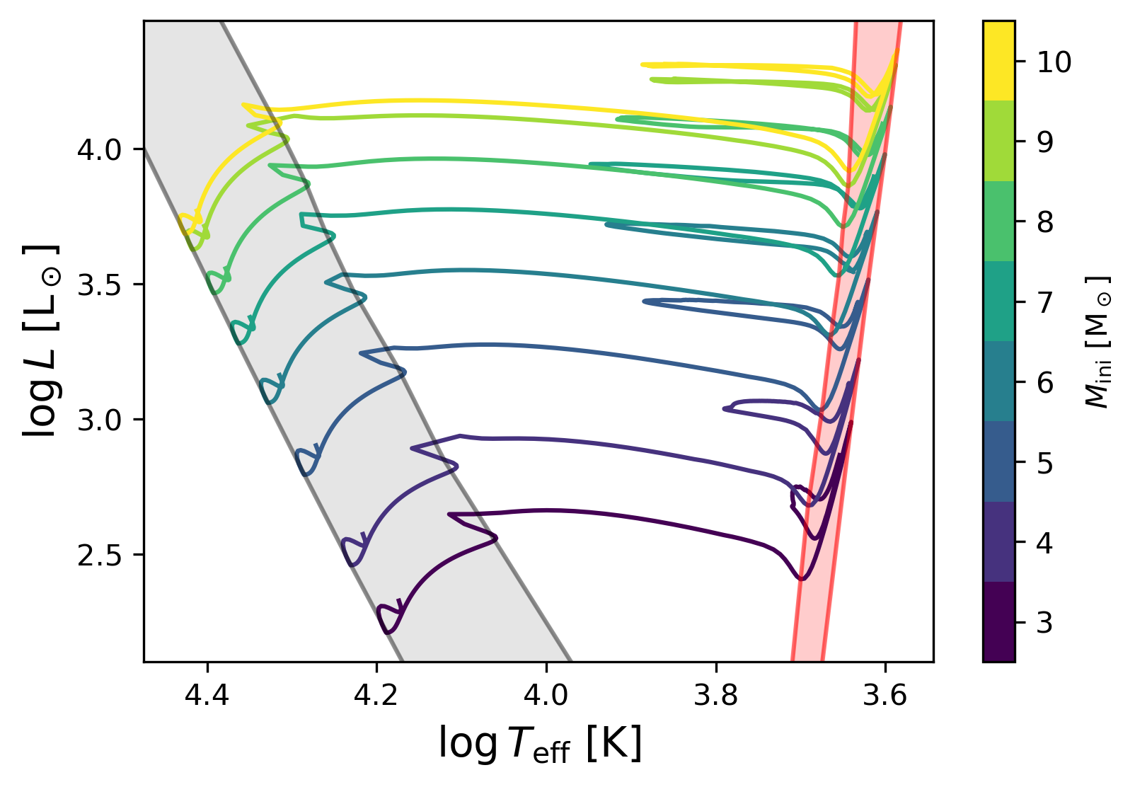
In this first part of the run, we want to stop the simulation before the star starts pulsating. A good way to do this is to terminate the run at the onset of core He burning. When the simulation is completed, your star will be at the tip of the Red Giant Branch (RGB), which is a mostly vertical structure on the Hertzsprung-Russell diagram (HRD), as may be seen on the figure below where the RGB is highlighted in red.

MESA has built-in stopping conditions for many common cases, but for practice we will implement this one ourselves in run_star_extras.f90!

Question: Check the MESA documentation of run_star_extras.f90 regarding the control flow. In which part of the evolutionary step does this stopping condition belong?

Now we have collected here some important information for you, that might help you with this task:

• At the end of the main sequence, hydrogen should be depleted in the core.
• To mark the start of helium burning, we can use the power generated by helium fusion.

Now try to code up that stopping condition! You can find some useful bits of code below if you need help with that.

While coding in the run_star_extras you will be using quantities and variables that are contained in the structure of the star.

To access all the information in the star’s structure you first need to define a pointer (which is already done in the code for you). You can find all the variables available in the stellar structure using the files in $MESA_DIR/star_data/public/! We’ll specifically use the variables in star_data_step_input.inc and star_data_step_work.inc.

s% center_h1      ! central H abundance
s% power_he_burn  ! power from He burning, in Lsun units

type (star_info), pointer :: s

log_of_number = safe_log10(number)

if (condition_you_want_to_meet) then
    what_happens
endif

if (condition_1 .and. condition_2) then
    what_happens
endif

Try and code it yourself, but if you are have some trouble don’t hesitate to ask for help or click on the answer below!

! ====== TODO: add stopping condition here! ======
if (s% center_h1 <= 1d-12 .and. safe_log10(s% power_he_burn) > 1d0) then
      extras_finish_step = terminate
      write(*, *) '===== you have reached the base of the RGB! ===='
      s% termination_code = t_extras_finish_step
end if
! ================================================

To check that everything is working correctly, let’s first compile the model using

./clean
./mk

If no errors pop up, you are all set! Now run the model using

./rn

During this first run you will see the star evolving through the main sequence and across the Hertzsprung gap to the base of the RGB. The second part of the simulation will start from this point.

3. Ah yes, the remix: stopping condition in the inlist_project

At this point, the star has reached the base of the RGB. Now we want it to evolve until the end of He burning. To that end, we need to choose and implement a different stopping condition!

Task 3.1: Comment or remove the previous stopping condition.

Open run_star_extras.f90 again and look for the stopping condition you just implemented. Once you find it, take extra care in commenting (or deleting) every line that you wrote!

Since you changed run_star_extras.f90, you also need to update the executable. In order to effectively remove the first stopping condition from the next part of the evolution, we need to delete the previous star file from the folder. Now make a new executable file using

./clean
./mk

Task 3.2: Setting a new stopping condition.

In this second part of the run, we want to stop the simulation when He is depleted in the core of the star. Luckily, in this case MESA provides a pre-made stopping condition for when the mass fraction of an isotope goes below a user-set value. Can you find it in the documentation?

Once you have found the right command, implement the stopping condition in your inlist.

In this case, we want to stop the simulation when the mass fraction of leftover Helium in the core goes below 1d-4.

   ! == TODO: add a stopping condition here! ==
   ! we want the second part of the run to stop when
   ! the mass fraction of he4 drops below 1d-4
   xa_central_lower_limit_species(1) = 'he4'
   xa_central_lower_limit(1) = 1d-4

Amazing! Now you are ready to continue your simulation!

Great, we have the second part of the run set up…but how do we continue without losing what we just computed?

4. Take two: ./re

A very powerful feature of MESA is the possibility to restart a simulation from previous steps in the evolution.

This lab is a perfect example of this: we have just run a simulation for a star that has reached the base of the RGB. If we want to evolve it further (like up to He depletion), there is no need to make a new simulation from scratch: restart the one you have just stopped!

The way to do it is by using photos files. These are custom binary files written by MESA, like ‘snapshots’ taken during the evolution of the star. You can find them in the photos/ directory.

Now we want to restart our simulation from the last photo MESA took at the end of the previous simulation.

Look into the output from your terminal; you should see something like this

save photos/x00000384 for model 384
termination code: extras_finish_step

If we want to restart from a specific photo we pass it to the re script like this:

./re x00000384

However, if you know you want to start from the most recent photo, you can simply call ./re.

With all that out of the way go ahead and restart your run from the most recently saved photo.

5: Oh no, the run stopped…

A few time steps into your run, the model should crash and leave you with an error message like:

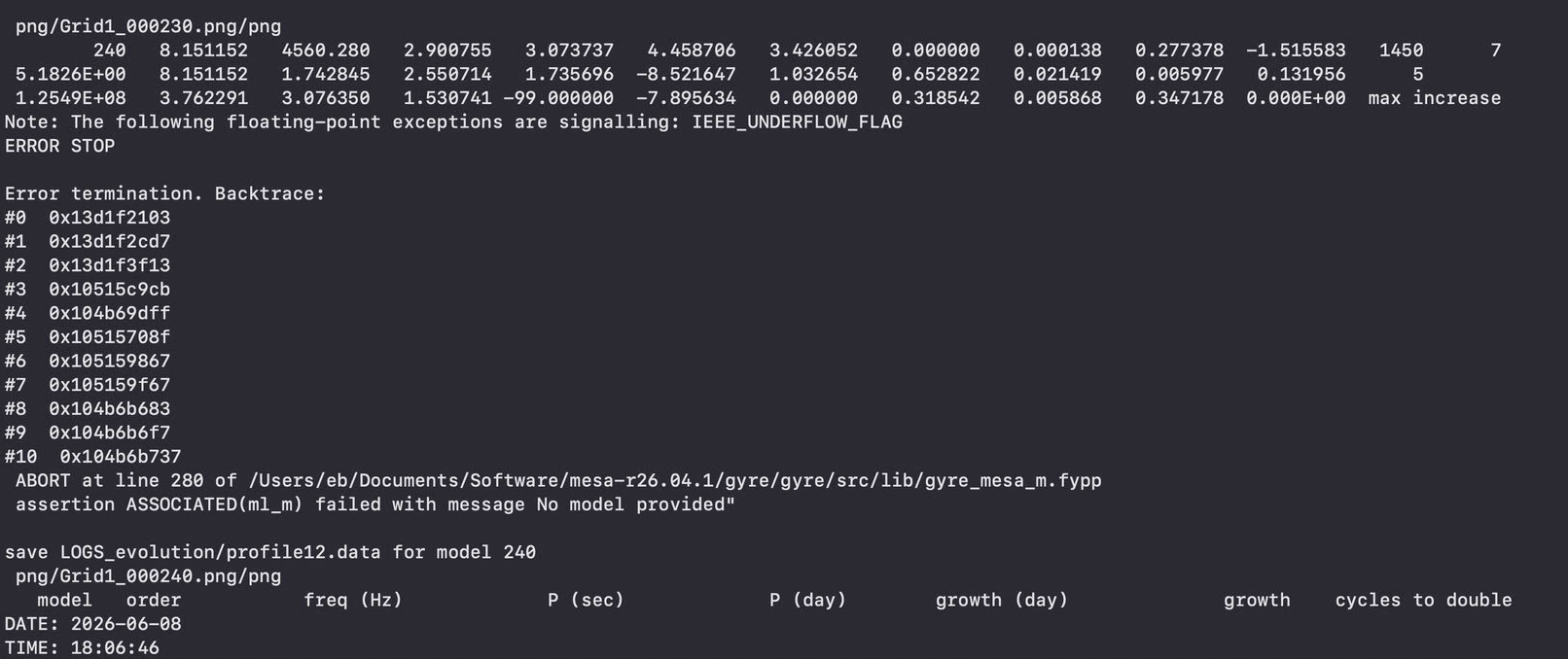
Although the first line of the error message points to a file in the MESA source code, the later error message tells us that the error is actually in run_star_extras during the extras_finish_step routine. To understand how to fix this, we need to look a bit deeper at the provided run_star_extras file.

This run_star_extras file does two important things: calls GYRE as MESA is running to save data to the history file and saves some .mod files with custom names and based on a custom criteria.

We’ll focus first on the GYRE portion. In previous labs, you used GYRE as a post-processing code on stellar structures saved by MESA and converted to a GYRE-readable format. There is also a way to run GYRE on-the-fly during the evolution, which is what we will use in this lab. In order to use GYRE in this way we have to load the GYRE library with the statement

   use gyre_mesa_M

at the top of the run_star_extras file. We also added a few variables to pass the values returned by GYRE from one run_star_extras routine to another. These variables are

   ! GYRE variables to write to history
   real(dp) :: F_period, F_growth
   real(dp) :: O1_period, O1_growth
   real(dp) :: O2_period, O2_growth

In addition to loading the GYRE library we also need to initialize GYRE and set some constants for GYRE to use. Since we only need to do this once per run, we use the extras_startup routine for this. This is mandatory any time you want to use GYRE within MESA. The code for this looks like

      ! Initialize GYRE

      call init('gyre.in')

      ! Set constants

      call set_constant('G_GRAVITY', standard_cgrav)
      call set_constant('C_LIGHT', clight)
      call set_constant('A_RADIATION', crad)

      call set_constant('M_SUN', Msun)
      call set_constant('R_SUN', Rsun)
      call set_constant('L_SUN', Lsun)

      call set_constant('GYRE_DIR', TRIM(mesa_dir)//'/build/gyre/src')

Scrolling down further to the data_for_extra_history_columns routine, you should see that here that we pass each of the columns we want to save. The mode information comes from the variables defined at the start of the file, and the photospheric composition is read directly from the model cell MESA identifies as the photosphere.

         names(1) = 'F_period'
         vals(1) = F_period

         names(2) = 'F_growth'
         vals(2) = F_growth

         names(3) = 'O1_period'
         vals(3) = O1_period

         names(4) = 'O1_growth'
         vals(4) = O1_growth

         names(5) = 'O2_period'
         vals(5) = O2_period

         names(6) = 'O2_growth'
         vals(6) = O2_growth

         names(7) = 'photosphere_X'
         vals(7) = s% X(s% photosphere_cell_k)

         names(8) = 'photosphere_Z'
         vals(8) = s% Z(s% photosphere_cell_k)

However, these values are not calculated here. Instead, we calculate them in the extras_finish_step function.

Let’s go back to the extras_finish_steproutine and see how that’s done, look specifically for the section marked by

! ======= Routines for the core helium burning part of the evolution ! ======

Right after this comment we set two logical variables, call_gyre and need_to_save_model, to .false. This is because we want to decide at run time when GYRE will be called and when we will save models. The logical variable in_gyre_region is used for the part of the evolution where we want denser output.

We then have a few lines of code which parse the x_integer_ctrl and x_ctrl values set in the inlist. This renaming isn’t strictly necessary, but it makes the code more legible.

      ! Save user specified parameters with meaningful names
      gyre_interval = s% x_integer_ctrl(1)! Sets how often to call GYRE in the inlist
      max_mode_num = s% x_integer_ctrl(1) ! Sets how many modes should be saved
      mode_l = s% x_integer_ctrl(1)       ! Sets l value of modes
      save_mod_Teff_limit = s% x_ctrl(1) ! Sets minimum Teff necessary to save a model

However, you might notice that the current code sets the mode-control variables to x_integer_ctrl(1), even though the inlist provides separate controls for them.

Task 5.1 Use the comments in inlist_project to correct max_mode_num and mode_l.

   ! Save user specified parameters with meaningful names
   gyre_interval = s% x_integer_ctrl(1)! Sets how often to call GYRE in the inlist
   max_mode_num = s% x_integer_ctrl(2) ! Sets how many modes should be saved
   mode_l = s% x_integer_ctrl(3)       ! Sets l value of modes
   save_mod_Teff_limit = s% x_ctrl(1) ! Sets minimum Teff necessary to save a model

We then zero out the variables that we saw used in data_for_extra_history_columns.

   ! Zero out period and growth rate information from previous step, if we don't call GYRE then values stay 0.
   F_period = 0d0
   F_growth = 0d0
   O1_period = 0d0
   O1_growth = 0d0
   O2_period = 0d0
   O2_growth = 0d0

The supplied inlist sets s% x_integer_ctrl(1) = 1, so GYRE is called every step in the dense-output part of the run. If you later increase this interval, the values from the previous GYRE call would otherwise persist on steps where GYRE was not actually called. By setting everything to zero we ensure that we only have results for time steps where GYRE was actually called.

The code then checks if we are in the part of the evolution where we want GYRE output. We want the GYRE region to begin when

1. We are in the core helium burning stage.
2. Models have logTeff above 3.66d0 (this ensures that these models work well for lab 2).

Inside this region, the history output, terminal output, and .mod file saves all follow the GYRE cadence, which is controlled by gyre_interval and set to 1 in the supplied inlist. Outside this region, history and terminal output return to every 10 models, and .mod file saving is disabled.

These checks are done by this bit of code:

   ! Check if in He burning and we're calling GYRE.
   in_gyre_region = s% center_h1 <= 1d-12 .and. &
      safe_log10(s% power_he_burn) >1d0 .and. logTeff > gyre_logTeff_min
   if (in_gyre_region) then
      save_mod_interval = gyre_interval
      s% history_interval = gyre_interval
      s% terminal_interval = gyre_interval
      if (gyre_interval > 0 .and. MOD(s% model_number, gyre_interval) == 0) then
         call_gyre = .true.
      end if
      if (save_mod_interval > 0 .and. MOD(s% model_number, save_mod_interval) == 0) then
         need_to_save_model = .true.
      end if
   else
      save_mod_interval = -1
      s% history_interval = 10
      s% terminal_interval = 10
   end if

Then, if we need to call GYRE there’s some further set up necessary. GYRE needs the structure variables from MESA in a specific format. Getting this format is a two-step process. First, we need to get the stellar structure data that will be passed to the GYRE pulsation code. This is accomplished with the star_get_pulse_data subroutine.

Task 5.2 This routine has three logical input parameters, take a moment to search the code base and try to figure out what each parameter controls.

$MESA_DIR/star/public/star_lib.f90: star_get_pulse_data => get_pulse_data, &

After getting the pulse data, we now need to put it into a form that GYRE can handle. The starter has a TODO in this part of run_star_extras; without this call, GYRE has no model to use and the run stops with the error shown above.

Task 5.3 Take a look at $MESA_DIR/gyre/public/gyre_mesa_m.f90 to see if you can figure out the correct subroutine to call.

call set_model(global_data, point_data, s%gyre_data_schema)

After making the changes for Tasks 5.1 and 5.3, rebuild the executable and restart again:

./clean
./mk
./re

We then write a header to the terminal so that you know what information is being printed, set a few parameters we’ll discuss in a moment and

call get_modes(mode_l, process_mode_cepheid, ipar, rpar)

As noted in the comments:

! The subroutine calls GYRE to find the modes.
! After each mode is found, it calls the subroutine process_mode_cepheid defined below
! Integer parameters are passed with ipar and real parameters are passed with rpar
! These two arrays allow us to pass information back and forth with the process mode subroutine
! However we choose to use the xtra#_array values that are a part of the star_info structure, so indexing is less confusing

We then move the information returned by GYRE to the variables used by data_for_extra_history_columns. In this setup, GYRE in MESA also prints some information to the terminal but again only once log_Teff = log10(T_eff/K) is greater than 3.66.

The last additional steps in this subroutine check whether we need to save a .mod file. The saved models go into mod_dir/; keep that directory because Lab 3 uses these saved models as starting points for nonlinear saturation runs. In the GYRE region, the model-save interval is temporarily set to gyre_interval, while x_ctrl(1) = 0d0 means the effective-temperature cut does not reject any of those saves.

6. Nice! Now let’s change the pgplot window during the run!

Ok you have started the final part of the run for your lab, but there is still plenty you can do! You might have already noticed from the MESA simulations in the previous days, that a pgplot panel with figures will pop up when you start running. Do you know you can change that while the model is running? Crazy!

Let’s take advantage of this awesome feature, shall we?

Task 6: Add the instability strip to the HRD

Since we are looking at the evolution of a Cepheid star, an extremely useful feature we can add to our HRD is the classical instability strip. In this region, stars usually pulsate, and we want to know if your model enters this phase or not.

Thankfully, MESA already provides a built-in command to show the two edges (respectively blue/hot and red/cool) of the instability strip to your HRD.

First, open inlist_pgstar with some text editor. Then paste this line into the file (where you put it is not strictly relevant).

show_HR_classical_instability_strip = .true.

In the next step of the evolution, you will see the two lines appear on the HRD on your screen. At some point during the run you should see something like this:

7. Hooray! You survived the setup - let’s talk science!

Now let’s take a look at the other panels, which contain some very interesting information, especially for the next labs.

During the evolution you should see something like this:

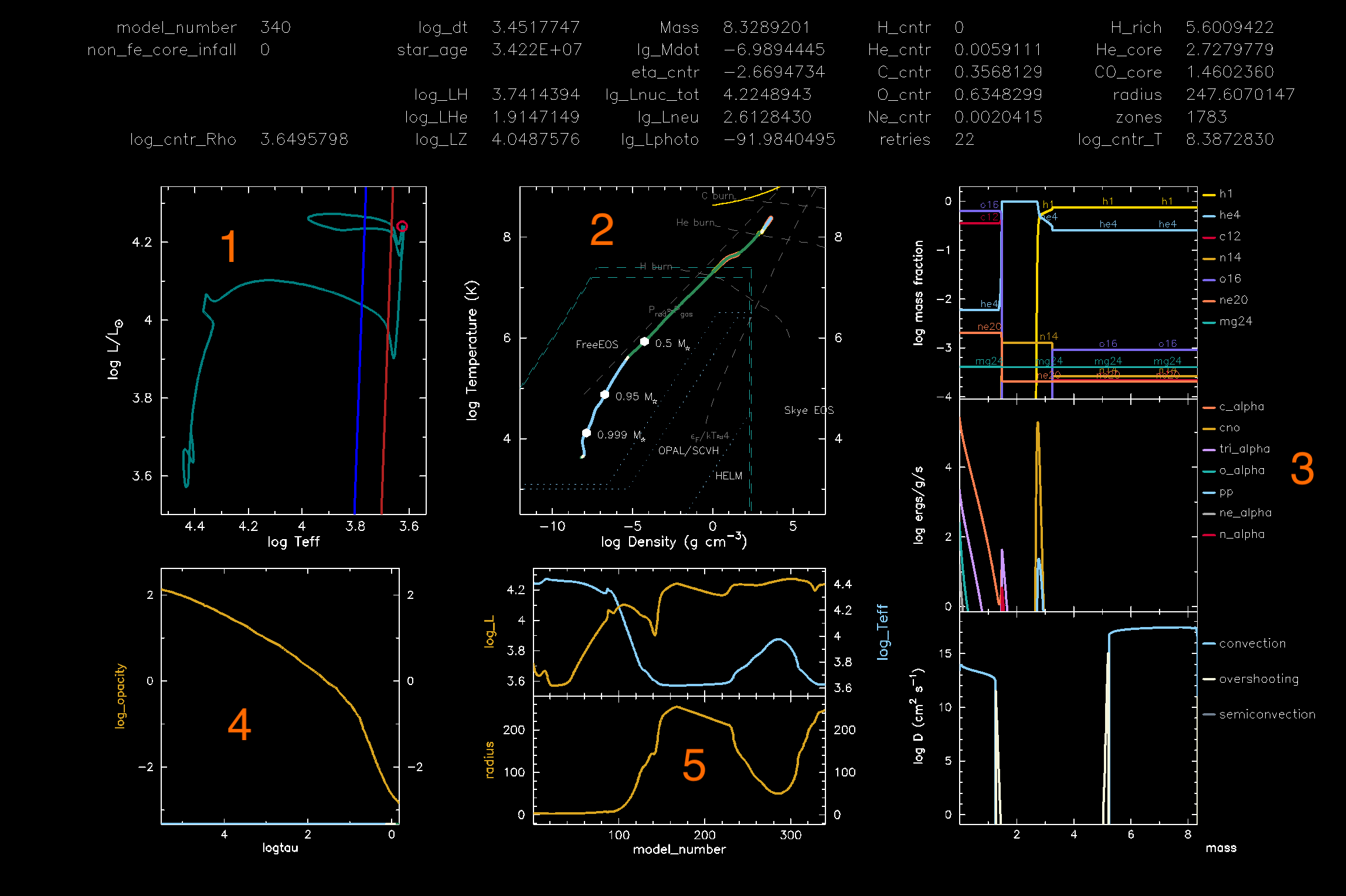There is a text summary plus 5 science panels:

1. HRD: This is the Hertzsprung-Russell diagram. The two additional lines are the edges of the Instability Strip, a region of the HRD where stars pulsate. What is your model doing right now? Is it entering the strip or not?

2. density/temperature: This is a radial density-temperature profile, showing the different regimes of the equations of state in which each point in the interior of a star is. Can you distinguish which end of the line is the core and which is the surface? How much does the temperature change from the core to the surface?

3. Combined panel: In this panel you can see 3 figures stacked on top of each other. From top to bottom, they show the chemical abundances in the interior of the star, the energy generation, and the internal mixing processes, all as a function of the mass coordinate. Where are the convective zones? Can you see any changes while the model is evolving?

4. opacity: In this plot you can see the value of opacity throughout the interior of the star. Note that the x-axis is a function of the logarithm of the optical depth. How is opacity changing in the star during the evolution? Can you link it to the energy transport mechanism? What happens to your opacity profile as your model enters the instability strip?

5. radius, temperature, and luminosity: Finally in this panel you can see how log_R, log_Teff, and log_L evolve with model number during the evolution of the star.

You might notice that even once your star has crossed into the instability strip, it doesn’t pulsate. Question: Why not?

8. To blue loop or not to blue loop? That is the question

After your simulation are completed, take a look at the last .png file that MESA saved, and compare it to those of the other people at your table. Can you answer the following questions? Share possible hypotheses with the folks at your table!

• Which masses make the cleanest blue loops?
• Which models actually enter the instability strip?
• How does the Cepheid candidate phase depend on mass?
• Which saved structures are the best starting points for Lab 2?

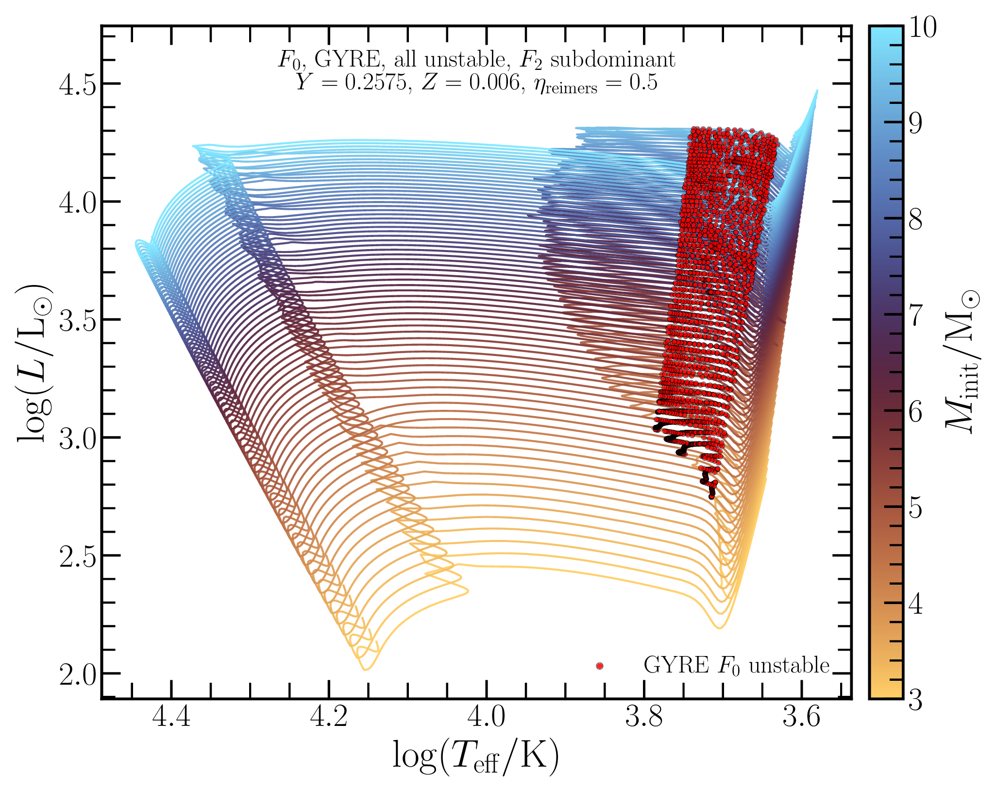
Solution example: GYRE-unstable Cepheid candidates (spoilers!)

The plot below shows the full Lab 1 grid after running GYRE in MESA. The colored tracks are grouped by initial mass. The overplotted points mark saved models where the GYRE fundamental mode is unstable, and where the second overtone is subdominant to the plotted mode. These are useful structures to compare when choosing Lab 2 RSP-LNA starting models.