Lab 3: The Hertzsprung Progression
Lab written by: Andy Santarelli (lead TA), Mathijs Vanrespaille (lead TA), Lynn Buchele, Sofia Mesini, and Ebraheem Farag (lecturer)
Background
In this lab you will take one of your saved Cepheid models from Lab 1, use a nonlinear pulsation setup to kick it into motion, and inspect the resulting waveform. Your goal is to identify where the bump appears in the cycle and combine your result with the rest of the class to reconstruct the Hertzsprung progression.
Many classical Cepheids show a distinctive “bump” in their waveform. The figure below shows a few examples of folded Cepheid light curves observed by the OGLE study.
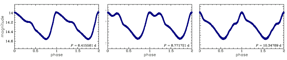
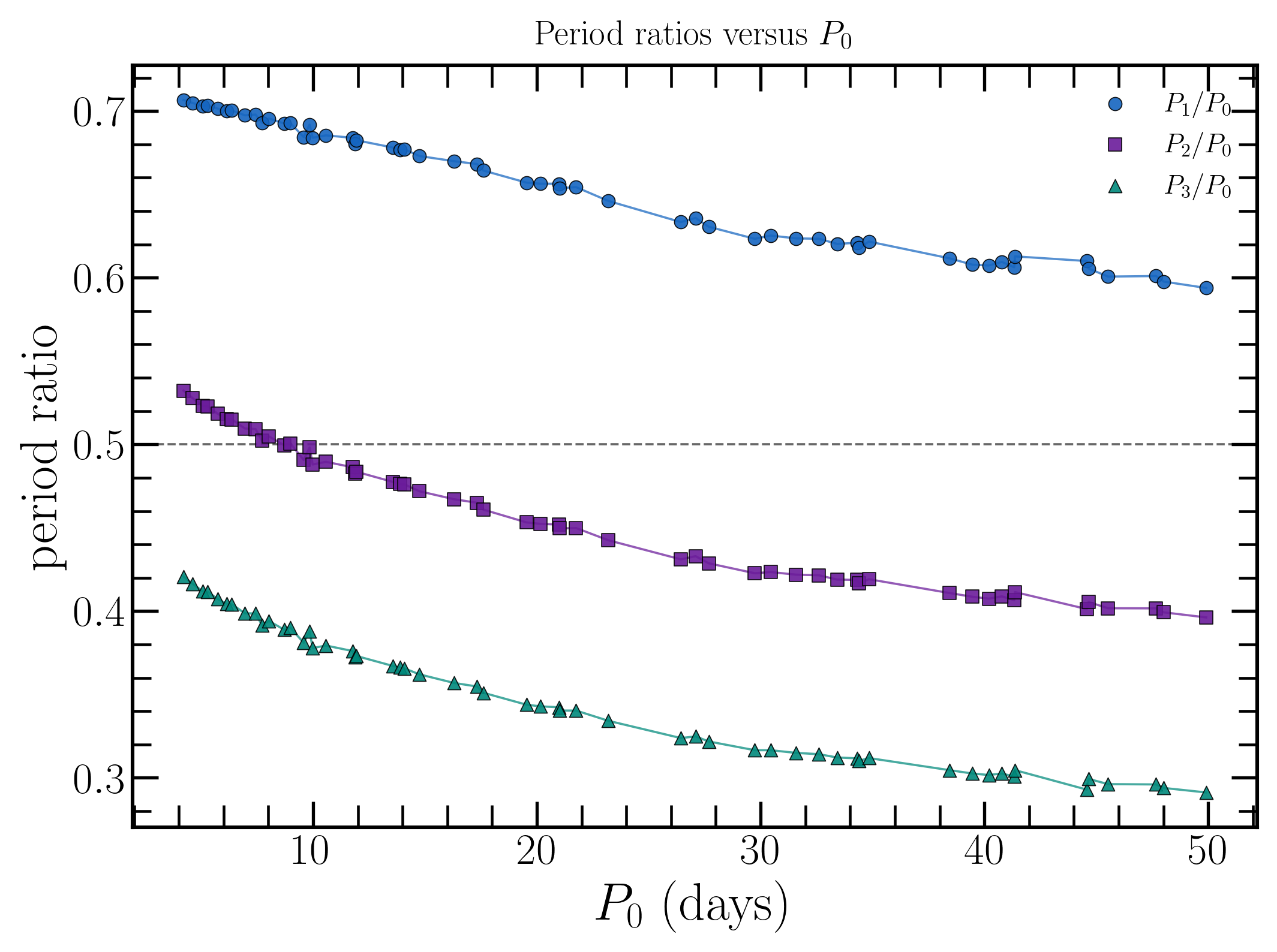
The location of that bump changes with the pulsation period. In the standard single mode picture, this is related to a near 2:1 resonance between the second overtone and the fundamental mode, so a useful quantity to keep in mind is
The linear nonadiabatic (LNA) plot below shows the overtone period ratios as a function of the fundamental mode period, . It shows why this ratio is useful: the second overtone ratio, , passes through the resonance range near the periods where bump Cepheids become most morphologically interesting.
As the stellar structure changes across the instability strip, the bump shifts from the descending branch, through the middle of the cycle, and onto the rising branch. In this lab, you will see that progression directly in nonlinear MESA models.
Science Goals
- Evolve a selected Cepheid model into a finite amplitude nonlinear pulsation.
- Measure the pulsation period and decide whether the model develops a bump.
- Compare the bump location with the rest of the class sample to reconstruct the Hertzsprung progression.
Lab Goals
- Choose a starting
.modfile from your Lab 1 output or the shared sample. - Run the nonlinear setup until the waveform is developed enough to classify.
- Record the period, bump location, and comments needed for the class comparison.
MESA Goals
- Load a saved Lab 1
.modfile into the nonlinear MESA star TDC setup. - Use a GYRE kick to seed the fundamental radial mode and start the pulsation on lab timescales.
- Use the history output and PGSTAR diagnostics to inspect the light curve, radius curve, velocity curve, and bump morphology.
Lab Directions
For this lab you will start from a good Cepheid model, run the nonlinear setup, inspect the waveform shape, and decide where the bump appears.
Setting up the work directory
Download lab3_work_dir.zip from this Google Drive, unzip it into some empty directory, and cd into the resulting lab3_work_dir/ directory. You’ll see that it already contains the inlists you will need. However, we need to provide TDC with a starting model to initialize the nonlinear run.
We want to use a Lab 1 .mod file, ideally the one you identified during Lab 2, whose GYRE fundamental mode is unstable and is growing faster than the second overtone: F_growth > 0 and F_growth > O2_growth. Ideally, the fundamental mode also grows faster than the first overtone, F_growth > O1_growth, and the model is closer to the red edge of the instability strip. If you cannot find a model with F_growth > O1_growth, use a redder model with F_growth > 0 and F_growth > O2_growth. Models closer to the blue edge are more likely to switch into an overtone during the nonlinear run.
Copy your Lab 1 .mod files into the Lab 3 work directory:
cp -r /path/to/your/lab1/mod_dir/ .Important
Keep your Lab 1 and Lab 3 runs in separate working directories.
Alternatively, you can download the models from the Lab 1 mod file solutions, which are grouped by mass. If you do not have a useful saved model ready to run, use the Lab 3 nonlinear start model files, which contains the selected .mod files used for the shared Lab 3 sample.
Important
Lab 3 uses a saved .mod file from Lab 1. It does not use a photos/ restart file from Lab 1.
Note
Depending on how your downloaded files were unpacked, you may need to fix permissions before opening or copying the model folders. If needed, you can use chmod on the extracted mass directory and its contents. Here is a guide to chmod if you need a refresher.
Task 1: Choose a Starting Model
Take a look inside mod_dir/. These are the saved stellar structures that Lab 3 can use.
The filenames are written in the form
modelNumber_currentMass_effectiveTemperature_luminosity.modIf you are using the Lab 3 nonlinear start model files instead of your own Lab 1 mod_dir/, the selected files have a longer name with the period and initial mass prepended. In those filenames, the final four underscore separated fields before .mod are still the Lab 1 model number, current mass, effective temperature, and luminosity.
Show Table 1: Optional example models for each mass
Table 1 lists one selected example saved model for each initial mass in the shared Lab 3 sample. These models were chosen from the redder side of the instability strip, visually about 10-30% of the plotted strip width in from the red edge.
If you do not have a useful saved model from Lab 1, use these Lab 3 nonlinear start model files. The downloaded filenames include the period and initial mass at the front; the final four underscore separated fields before .mod are still the Lab 1 model number, current mass, effective temperature, and luminosity.
| Minit | model | M | Teff | L | P0 | growth |
|---|---|---|---|---|---|---|
| 3.9 | 358 | 3.854 | 5553 | 1049 | 4.2104 | 0.002001 |
| 4 | 405 | 3.9511 | 5522 | 1167 | 4.6231 | 0.0039758 |
| 4.1 | 408 | 4.0477 | 5488 | 1287 | 5.055 | 0.0042498 |
| 4.2 | 406 | 4.1454 | 5517 | 1413 | 5.2906 | 0.0073861 |
| 4.3 | 383 | 4.2429 | 5480 | 1541 | 5.7269 | 0.013038 |
| 4.4 | 417 | 4.3406 | 5461 | 1674 | 6.1264 | 0.0084876 |
| 4.5 | 382 | 4.4381 | 5490 | 1822 | 6.3553 | 0.024002 |
| 4.6 | 362 | 4.5354 | 5434 | 1967 | 6.9485 | 0.014852 |
| 4.7 | 337 | 4.6313 | 5358 | 2127 | 7.7118 | 0.014443 |
| 4.8 | 326 | 4.7295 | 5492 | 2302 | 7.4145 | 0.040702 |
| 4.9 | 325 | 4.8268 | 5450 | 2480 | 8.0179 | 0.018694 |
| 5 | 324 | 4.9236 | 5400 | 2661 | 8.6847 | 0.030977 |
| 5.1 | 320 | 5.0218 | 5265 | 2834 | 10.08 | 0.052909 |
| 5.2 | 245 | 5.1333 | 5225 | 2665 | 9.5959 | 0.0054239 |
| 5.3 | 248 | 5.2322 | 5382 | 2858 | 8.9897 | 0.05625 |
| 5.4 | 320 | 5.3124 | 5484 | 3491 | 9.9291 | 0.1059 |
| 5.5 | 251 | 5.427 | 5275 | 3254 | 10.573 | 0.037957 |
| 5.6 | 322 | 5.5062 | 5317 | 3927 | 12.083 | 0.10817 |
| 5.7 | 248 | 5.6213 | 5230 | 3689 | 11.891 | 0.05177 |
| 5.8 | 251 | 5.72 | 5296 | 3911 | 11.745 | 0.062656 |
| 5.9 | 330 | 5.7985 | 5292 | 4654 | 13.561 | 0.025517 |
| 6 | 336 | 5.8957 | 5294 | 4931 | 14.053 | 0.041635 |
| 6.1 | 249 | 6.012 | 5228 | 4661 | 13.889 | 0.059128 |
| 6.2 | 246 | 6.1102 | 5195 | 4918 | 14.755 | 0.073988 |
| 6.3 | 328 | 6.1851 | 5233 | 5759 | 16.391 | 0.077703 |
| 6.4 | 323 | 6.2831 | 5175 | 6056 | 17.802 | 0.15068 |
| 6.5 | 324 | 6.3794 | 5237 | 6356 | 17.523 | 0.1441 |
| 6.6 | 331 | 6.476 | 5111 | 6618 | 19.566 | 0.024603 |
| 6.7 | 322 | 6.5724 | 5115 | 6966 | 20.508 | 0.065634 |
| 6.8 | 330 | 6.6685 | 5099 | 7293 | 21.366 | 0.097282 |
| 6.9 | 338 | 6.7661 | 5138 | 7619 | 21.028 | 0.036579 |
| 7 | 337 | 6.8676 | 5123 | 7931 | 22.006 | 0.09578 |
| 7.1 | 250 | 6.9844 | 5015 | 7855 | 23.684 | 0.20211 |
| 7.2 | 335 | 7.0584 | 4934 | 8514 | 27.117 | 0.092097 |
| 7.3 | 331 | 7.1539 | 4955 | 8920 | 27.551 | 0.077469 |
| 7.4 | 247 | 7.2753 | 4902 | 9037 | 28.158 | 0.10547 |
| 7.5 | 247 | 7.3715 | 4866 | 9451 | 30.562 | 0.1905 |
| 7.6 | 333 | 7.4452 | 4895 | 10035 | 31.284 | 0.11722 |
| 7.7 | 335 | 7.5406 | 4889 | 10478 | 32.444 | 0.13049 |
| 7.8 | 333 | 7.6346 | 4904 | 11049 | 33.29 | 0.12951 |
| 7.9 | 337 | 7.7362 | 4878 | 11279 | 34.351 | 0.14845 |
| 8 | 247 | 7.8529 | 4869 | 11810 | 34.674 | 0.0051594 |
| 8.1 | 338 | 7.9267 | 4913 | 12322 | 35.018 | 0.076185 |
| 8.2 | 328 | 8.0193 | 4933 | 12882 | 35.755 | 0.15895 |
| 8.3 | 335 | 8.1155 | 4821 | 13261 | 40.443 | 0.18995 |
| 8.4 | 326 | 8.2107 | 4872 | 13828 | 39.582 | 0.2245 |
| 8.5 | 328 | 8.3075 | 4843 | 14273 | 41.582 | 0.26344 |
| 8.6 | 336 | 8.4078 | 4835 | 14753 | 42.817 | 0.24125 |
| 8.7 | 333 | 8.5029 | 4879 | 15318 | 42.194 | 0.30491 |
| 8.8 | 325 | 8.5939 | 4845 | 15842 | 44.594 | 0.29118 |
| 8.9 | 328 | 8.6872 | 4925 | 16484 | 42.687 | 0.30096 |
| 9 | 331 | 8.7831 | 4830 | 16931 | 47.224 | 0.31013 |
| 9.1 | 331 | 8.8803 | 4883 | 17606 | 46.332 | 0.34419 |
| 9.2 | 264 | 8.9989 | 4846 | 18752 | 48.428 | 0.036197 |
| 9.3 | 267 | 9.0907 | 4827 | 19394 | 51.824 | 0.39692 |
| 9.4 | 330 | 9.1655 | 4871 | 19250 | 49.314 | 0.31887 |
Question: What would make an interesting model to simulate in further detail using TDC?
Click here to open the hint
Choose a model that:
- is in the Cepheid part of the blue loop
- is on the redder side of the instability strip, visually about 10-30% of the plotted strip width in from the red edge
- preferably showed positive fundamental mode growth in Lab 1
- is part of the shared class sample, so different groups cover different periods
For this lab, the redder edge is a safer place to start because the nonlinear run is more likely to stay in the fundamental mode instead of switching into an overtone. Table 1 lists the redder selected models used for the shared Lab 3 sample. The distance from the red edge is a visual guide on the HR diagram, not a formal temperature criterion.
An especially good choice is a model with a relatively large fundamental mode growth rate. If you also estimated that is close to , that makes the model even more interesting for this lab.
This choice is partly about mode selection. A model can have more than one linearly unstable radial mode. The final nonlinear state is then not determined by the largest linear growth rate alone. The initial perturbation, saturation, damping, and mode coupling can all matter. For this lab we deliberately choose models and kicks that favor a stable fundamental mode pulsator.
Note
These .mod files come from the second part of Lab 1, after you restarted the evolution with ./re and let the star pass through the Cepheid phase while GYRE was running during the evolution.
Caution
In Lab 1, restarting with ./re appends to the existing history.data file. That means model numbers in the history output may not increase monotonically. If you go back to Lab 1 to recover period or growth information for a saved model, keep that in mind while matching rows in history.data.
Task 2: Edit the Lab 3 Inlist
Open inlist_pulses in your editor.
Find the line
load_model_filename = 'mod_dir/YOUR_MODEL.mod'For your first run:
- update
load_model_filenameso it points to the model you copied into your localmod_dir/
Note
In this setup, MESA loads the saved stellar structure, removes the core, remeshes the envelope for time dependent convection, and then uses a GYRE kick to seed the fundamental radial mode.
Task 3: Choose and set an initial kick
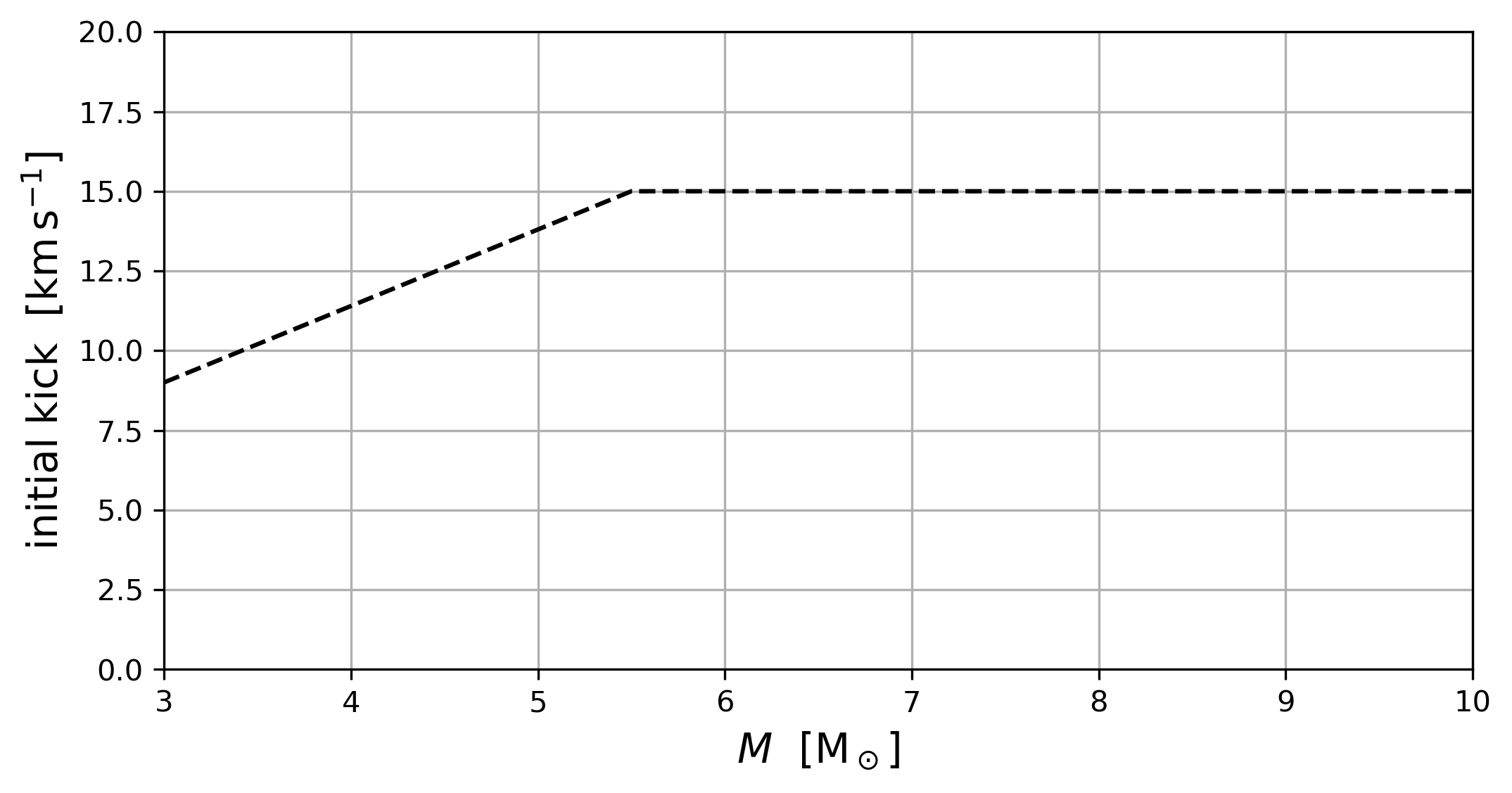
It can take a very long time for a MESA TDC model to start pulsating “naturally”. Therefore, we get the pulsation going by giving the model an initial kick. To that end, the eigenfunction of the fundamental pulsation mode, which expresses how the star is perturbed by the pulsation, is computed using GYRE and scaled to an initial kick velocity that you choose.
The closer this kick is to the final pulsational radial velocity, the faster the bump in the light curve will develop. From the figure below, read off a reasonable initial kick for your chosen model.
Now add this value into your inlist_pulses. Question: Can you find which variable stores the initial kick?
Hint: where to look
There exists no dedicated field for the initial kick of a Cepheid in MESA, so the official MESA documentation won’t be of help.
Instead, think about which variables one uses when defining custom quantities in a MESA inlist.
Answer
Find and update this line in the &controls of inlist_pulses:
x_ctrl(6) = 10d0 ! initial vsurf (kms)Caution
In real scientific applications, it is safest to give the Cepheid a small initial kick and give the model a long time to converge to its final value. In this lab, however, it is okay to risk using a larger kick to save time.
The kick is also a mode selection choice. Here we seed the fundamental radial mode because the class goal is the fundamental mode Hertzsprung progression. For a production calculation, especially near regions where multiple modes are unstable, you would test that the final state does not depend strongly on the exact kick amplitude or on which mode was initially excited.
Task 4: Compile and Run the Model
First compile the work directory:
./clean
./mk
Tip
Make sure you are running inside your extracted Lab 3 work directory before calling ./clean, ./mk or ./rn.
If the compilation succeeds, start the nonlinear run:
./rnWarning
Be warned, this will likely take at least 10 minutes. In the meantime, read through the tasks below. They explain what signs to look for when deciding whether the run has gone far enough to classify the bump. If you reach the end of these tasks and your waveform has not stabilised, take a look at the If You Are Still Waiting on a Run section.
Task 5: Watch the Diagnostics
The PGSTAR panels are by far the most important diagnostics for this lab. For most students, they already summarise nearly everything that matters for deciding whether the pulsation is developing well and whether a bump is visible.
If you want to know where the supporting output is written, the run also saves files in:
png_pulsation/LOGS_pulsation/photos/
Tip
Compare your PGSTAR animation with the other students at your table. This is often the fastest way to see how different models behave.
Task 6: Decide Whether the Run Is Good Enough
For the purpose of this lab, the run is useful once you can see that the kick has produced a coherent pulsation and the amplitude is either:
- still clearly growing
- or close to a repeating finite amplitude cycle
In the drop down, we provide some information on what standard should be applied to research quality nonlinear runs. Feel free to read this after starting your model.
Standards for coherent pulsations in research quality runs
For a research quality nonlinear pulsation calculation, the standard is stricter that what we have used in this lab. A true limit cycle means the initial transient has died away and the model has settled into a repeating finite amplitude pulsation. In practice, you would check the last several cycles and look for:
- a stable period from one cycle to the next
- stable maximum and minimum radius, luminosity, magnitude, and velocity
- no obvious secular drift in the waveform or bump phase
growthorKE_growth_avgclose to zero on average, because the pulsation is no longer growing or decaying
Positive growth is useful early in the run because it tells you the kick has excited a mode that is growing, but positive growth by itself does not mean the model has reached a limit cycle. It means the finite amplitude pulsation is still developing.
In this lab, we are using a looser practical standard. You do not need to prove that the model has reached a fully converged limit cycle. You only need a developed enough waveform to identify where the bump appears in the cycle.
The limit cycle test above is also specific to stable single mode pulsation. If a model settles into two persistent periods, switches mode, alternates cycle shapes, or keeps changing in a structured way, that is not just a failed single mode limit cycle. It may be a different nonlinear solution. In real work you would report that behavior, check whether it is physical or numerical, and then decide whether the model belongs in a single mode Cepheid sample.
Signs that the run is doing the right thing:
growthis positive for at least part of the rundelta_R,delta_logL, ordelta_Magare no longer consistent with numerical noise- the light, radius, or velocity curves begin to repeat from cycle to cycle
You can see an example of healthy, developed pulsation below.
Show PGSTAR pulsation example animation
The four panels labeled with a red number are the most relevant. They show:
- Hertzsprung-Russell diagram. We expect an ellipsoidal path for a purely sinusoidal waveform without a bump. In this example however, you can see a downward kink around .
- effective temperature variation over time in blue and luminosity variation in solar luminosity over time, also called the light curve, in yellow. This example is clearly not purely sinusoidal as the peak is too thin and there’s a subtle bump just before the peak. Any bumps are usually relatively easy to identify in this panel. You can see other examples of these light curves in the figure in the introduction or at the OGLE catalog.
- radial variation and surface radial velocity over time in yellow and blue, respectively. Once again, neither curve is sinusoidal, although the bump is not clearly visible here.
- radial velocity profile against optical depth as a proxy of depth from the surface. The initial kick should be plainly visible here after a few hundred time steps.
Signs that you should stop and rethink:
- the run exits immediately
- the model never develops a clear periodic signal
- the waveform looks obviously pathological rather than pulsational
Important
You do not need a perfect production quality nonlinear model. You only need a waveform that is good enough to classify the bump.
Note
If you want a slightly more quantitative rule of thumb, compare the last few cycles. For this lab, it is enough if the changes between cycles in quantities such as delta_R, delta_logL, delta_Mag, or KE_growth_avg are getting smaller and the plotted waveform begins to repeat cleanly. For a science quality limit cycle, you would keep running until those diagnostics are nearly stationary and growth or KE_growth_avg is close to zero rather than still clearly positive.
What if I accidentally ended my run too early?
If the run stops but has already written restart photos, you can continue from the most recent one:
./reTo restart from a specific photo file:
./re photo_nameThis is useful if the model is progressing normally but simply needs more cycles before the bump becomes easy to classify.
Just as in Lab 1, these photos/ files are for continuing your own run on your own machine.
Bonus task: modifying the radial velocity profile
If the optical depth as a proxy of distance to the surface in panel 4 confuses you, you can alter the x axis to your liking (radius, mass, zone number…). To do so, update Profile_Panels3_xaxis_name in inlist_pgstar. You need to give it the name of a column in your profile output, so check profile_columns.list to see all the options.
Depending on what quantity you pick, you may also have to alter the limits of the x axis using Profile_Panels3_xmin and Profile_Panels3_xmax. The default plot reverses the x axis; you can disable that by setting
Profile_Panels3_xaxis_reversed = .false.Task 7: Inspect the Waveform
Now look at the waveform and decide where the bump appears in the cycle.
Start with the PGSTAR plot. For almost everyone, this will be the easiest and clearest place to identify the bump.
If you want to check what you are seeing, you can also look at:
- the saved plots in
png_pulsation/ - the time series in
LOGS_pulsation/history.data
If possible, inspect more than one diagnostic. The bump is often easiest to see in a light curve in luminosity or delta_Mag, but the radius and surface velocity curves can help you decide whether a feature is real.
Use the following simple classification:
descending branch: the bump appears after maximum light while the curve is fallingmiddle: the bump is near the middle of the cycle and not clearly tied to either branchrising branch: the bump appears before maximum light while the curve is risingno clear bump: use this only if the waveform is genuinely ambiguous
Tip
Do not spend too long debating a borderline case. If the bump is ambiguous, record that uncertainty and move on.
Solution examples: nonlinear light curves across period (spoilers!)
The movie below is selected from the period limited nonlinear grid and is phased so that maximum V band light is at phase 0. It shows two pulsation cycles so the bump motion is easier to follow as the phased
and
curves change across the nonlinear Cepheid sample.
The plotter used to generate this movie is available here.
Task 8: Record Your Result
Add one row for your successful model to the shared class table.
At minimum, record:
- model filename
- initial mass
log Landlog T_eff, if available from Lab 1- fundamental period
- whether the pulsation was clearly established
- bump classification
- a short note such as
clear bump,weak bump, orneeded restart
Once the class table starts to fill up, switch to the “Lab 3: Sorted by Period” tab on the google sheets and look for the bump progression across the sample.
Questions for Discussion
As the class table fills in, discuss these questions at your table:
- how does bump location change with period?
- where does the bump move from the descending branch to the rising branch?
- does the class sample support the idea that the morphology is tied to the resonance?
- what finite amplitude information does the TDC waveform add beyond the Lab 2 periods and growth rates?
- did any model show behavior that was not cleanly single mode, such as overtone selection, alternating cycles, or a waveform that did not settle?
If You Are Still Waiting on a Run
These TDC runs can take a long time to converge, often more than 10 minutes. If your model is still running and you have some idle time, use that time to do one or more of the following:
- review your Lab 2 notes and make sure your expected period is written down
- look at the shared class table and decide which period range is still undersampled
- inspect the output files you already have and make a preliminary guess about the bump
- compare what you are seeing in PGSTAR with what appears in
history.data
Task 9 (BONUS): If You Have Extra Time
If your group finishes the core lab early, here are the most useful next steps:
- compare your TDC result directly with the linear information you already gathered in Lab 2
- look more carefully at how the bump appears in luminosity, radius, and velocity together
- compare your PGSTAR animation with the other students at your table
- make a movie of your PGSTAR output
You do not need to complete all of these. Pick the next one that feels most useful.
Option 1: Compare Back to Lab 2
If you completed Lab 2, compare your nonlinear result with the linear information you already had for the same model.
Ask yourself:
- did a model with positive linear growth turn into a useful nonlinear pulsator?
- is the nonlinear period similar to the period you expected from the linear analysis?
- did the model you thought would be interesting actually produce a clear bump?
If you also estimated where is closest to , compare that expectation with the waveform shape you actually see in the TDC run.
Option 2: Compare Different Diagnostics
If you have a clearly pulsating model, compare the bump location in:
- behavior related to luminosity
- radius
- surface velocity
You may find that the bump is easier to identify in one diagnostic than another. Record that in your notes if it helps explain your classification.
Option 3: Compare with Other Students at Your Table
If several people at your table have useful runs, compare them directly:
- do the bumps appear in different parts of the cycle?
- do the PGSTAR animations suggest a smooth progression across period?
- which models develop the clearest bump?
Option 4: Making a movie
Isn’t that animated PGSTAR window neat? Unfortunately, it vanishes once you end the run. Luckily, a bunch of .png files are output by MESA, which can be used to recreate the animated PGSTAR plots. You could either flick through them in an image viewer or combine them into a proper movie. MESA includes tools to make such movies. To do so, run the following in your terminal:
images_to_movie "png_pulsation/*.png" my_Cepheid_movie.mp4Tip
This images_to_movie command lives in the MESA SDK. If the command above ever fails, check that the SDK is initialised using echo $MESASDK_ROOT.
Troubleshooting
The run cannot find the model file
Check that:
- the file really exists inside
lab3_work_dir/mod_dir/ load_model_filenamematches the filename exactly- you are running from inside
lab3_work_dir/
The run builds, but the pulsation never becomes obvious
Try these in order:
- verify that you chose a genuine Cepheid candidate from Lab 1
- switch to a model that has a larger fundamental mode growth rate in the Lab 2 spreadsheet
- restart with
./reand let it continue longer - switch to a fallback model rather than spending the whole lab debugging one difficult case
I am not sure whether I am seeing a real bump
Compare more than one diagnostic:
- light curve in luminosity or
delta_Mag - radius variations
- surface velocity
If the same feature appears consistently in more than one place, it is more likely to be real. If not, mark the case as uncertain and move on.
Bonus coding task: average the light curve over one cycle
If you would like a more coding focused extension, modify run_star_extras so that it measures a cycle averaged quantity from the nonlinear light curve and compares that average with the corresponding static value from the original model.
You can find a complete set of Lab 3 bonus solutions with these source changes already made. As with the starter, you still need to copy in a .mod file and update load_model_filename.
One possible version of this task is:
- identify one full pulsation cycle after the model has reached a reasonably repeatable waveform
- measure a quantity over that cycle, such as luminosity or magnitude
- compute the time average over the cycle
- compare that cycle averaged value with the static value from the original stellar model
For example, you might compare:
- cycle averaged luminosity versus the original static luminosity
- cycle averaged magnitude versus the magnitude implied by the static model
Note
A simple arithmetic average over output points is not always the same as a true time average if the output sampling is uneven. A better version of this task is to weight the average by the timestep or by the time interval between samples.
Here is one reasonable way to implement this:
Step 1: Find the relevant source files
The most useful files to inspect are:
src/run_star_extras.f90src/run_star_extras_TDC_pulsation.incsrc/run_star_extras_TDC_pulsation_defs.inc
The existing Lab 3 setup already computes per cycle quantities such as:
perioddelta_logLdelta_MagKE_growth_avg
and writes them out through the extra history column machinery. That makes this a natural place to add one or two more derived quantities.
Step 2: Choose what you want to average
Start with one quantity only. Good choices are:
- luminosity
log_L- a magnitude like quantity
The simplest first version is to average luminosity over one completed pulsation cycle.
Step 3: Decide what you will compare against
Pick the corresponding static quantity from the original model. For example:
- cycle averaged luminosity compared with the model luminosity before the nonlinear pulsation becomes large
- cycle averaged magnitude compared with the magnitude implied by the static luminosity
You do not need to design a perfect scientific definition here. The point is to compare a static value with the value implied by the nonlinear cycle.
Step 4: Accumulate the average over one cycle
As the run advances, keep track of:
- the value of the quantity you are averaging
- the elapsed time associated with each sample
- the running weighted sum over the current cycle
- the total elapsed time over the current cycle
In other words, your code should conceptually build something like
over one pulsation cycle.
Tip
If you want a simpler first attempt, you can average over the samples within one cycle without time weighting. Just be clear in your notes that this is an approximation.
Hint for Step 4: where could you store the running sums?
One natural place is src/run_star_extras_TDC_pulsation_defs.inc, where the Lab 3 setup already stores period related quantities such as period, delta_logL, and delta_Mag.
You could add a few new variables there, for example:
- a running weighted sum
- a running total time
- the most recent cycle averaged value
- the difference between the cycle average and the static value
Then update those variables during the evolution in the same part of the code where the period related diagnostics are already being assembled.
Partial solution for Step 4: example accumulator variables
One possible pattern is to add a few variables to src/run_star_extras_TDC_pulsation_defs.inc, for example:
      real(dp) :: cycle_sum_L_dt, cycle_sum_dt
      real(dp) :: cycle_avg_L, cycle_avg_L_minus_static
      real(dp) :: static_L
Here the idea is:
cycle_sum_L_dtstores the running weighted sumsum(L * dt)cycle_sum_dtstores the running sumsum(dt)cycle_avg_Lstores the final cycle averaged luminositycycle_avg_L_minus_staticstores the comparison with the static model valuestatic_Lstores the reference luminosity from the starting model
You do not have to use exactly these variable names, but keeping the names explicit will make your code much easier to debug.
Step 5: Reset the accumulators at the start of a new cycle
The existing pulsation code already keeps track of completed cycles and period level information. Use that logic to decide when one cycle has ended and the next has begun.
At the end of each completed cycle:
- compute the average
- save the result somewhere
- reset the running sums for the next cycle
Hint for Step 5: where is the existing cycle logic?
Look in src/run_star_extras_TDC_pulsation.inc, especially in the code that already updates:
num_periodsperioddelta_Rdelta_logLdelta_Mag
That is the part of the setup that already knows when one pulsation cycle has been completed.
Partial solution for Step 5: example update and reset logic
At each timestep, you could accumulate your weighted sums with something like:
         cycle_sum_L_dt = cycle_sum_L_dt + s% L(1) * s% dt
         cycle_sum_dt   = cycle_sum_dt   + s% dt
Then, when the existing period logic determines that one full cycle has been completed, you could compute and store the average:
         if (cycle_sum_dt > 0d0) then
            cycle_avg_L = cycle_sum_L_dt/cycle_sum_dt
            cycle_avg_L_minus_static = cycle_avg_L - static_L
         end if
After saving the result for that completed cycle, reset the accumulators:
         cycle_sum_L_dt = 0d0
         cycle_sum_dt   = 0d0
This is only a sketch, but it shows the basic structure:
- accumulate during the cycle
- compute the average at cycle end
- reset for the next cycle
Step 6: Expose the new quantity in the history output
Once you have computed your new cycle averaged quantity, add it to the custom extra history columns so it appears in history.data.
That means updating the part of the code that currently exports values like:
periodgrowthdelta_Rdelta_Mag
You can either:
- replace one of the less important bonus outputs for your experiment, or
- increase the number of extra history columns and append your new quantity
Hint for Step 6: which routines control the extra history output?
The relevant routines are:
TDC_pulsation_how_many_extra_history_columnsTDC_pulsation_data_for_extra_history_columns
These are in src/run_star_extras_TDC_pulsation.inc.
If you add new output columns, remember to update both:
- the number of extra columns
- the names and values written into those columns
Partial solution for Step 6: example history column changes
Suppose you want to add two new history columns:
- the cycle averaged luminosity
- the difference between that value and the static luminosity
Then one possible change is:
TDC_pulsation_how_many_extra_history_columns = 14instead of 12.
Then append the new columns in TDC_pulsation_data_for_extra_history_columns, for example:
         names(i) = 'cycle_avg_L'; vals(i) = cycle_avg_L; i=i+1
         names(i) = 'cycle_avg_L_minus_static'; vals(i) = cycle_avg_L_minus_static; i=i+1
Make sure that:
- the number of columns matches the number of values you write
- the names are short enough to be readable in
history.data - the quantities are in units you understand when you interpret them later
Step 7: Recompile and rerun
Because this bonus task edits source include files, rerun both ./clean and ./mk before continuing. A plain rebuild can miss changes in included source files.
If you want to start and kick a new TDC model after editing the Fortran source:
./clean
./mk
./rn
If you want to continue from a previously saved TDC run after recompiling:
./clean
./mk
./re
Step 8: Compare the nonlinear average with the static value
Once your new quantity appears in the output, compare:
- the cycle averaged value obtained with TDC
- the corresponding static value from the original model
You can do this for one cycle or for several successive cycles if the run is still evolving.
Step 9: Interpret what you find
Write down a short conclusion:
- are the two values nearly the same?
- is there a systematic offset?
- does the offset shrink or grow as the pulsation settles?
- does averaging luminosity directly give a different answer than averaging a magnitude like quantity?
Tip
Keep this as a bonus task. The goal is not to build a perfect analysis pipeline, just to explore whether the nonlinear cycle average differs in an interesting way from the static model value.
Suggested Reading
- OGLE Atlas of Variable Star Light Curves, classical Cepheids
- OGLE Atlas of Variable Star Light Curves, Type II Cepheids
- Farag et al. 2026, self-consistent nonlinear classical Cepheid pulsations during stellar evolution with MESA
- Smolec 2014, mode selection in pulsating stars
- Bono, Marconi, and Stellingwerf 2000, the Hertzsprung progression
- Marconi et al. 2024, the Hertzsprung progression of classical Cepheids in the Gaia era