Lab 1: Gyrochronology

Authors: Joey Mombarg (lead TA), Niall Miller, Eliza Frankel - Lecturer: Yaguang Li — MESA Summer School 2026, Tetons, Wyoming

Special thanks to the Monday Lab of the MESA Summer School 2025 at KU Leuven for the template, and Nick Saunders for sharing his MESA setup used in Saunders et al. (2024).

In this lab, you will learn how to set up a MESA model from scratch, monitor the run, and customize its output.

Introduction

Stars with a (significant) convective envelope experience a braking of their rotation velocity at the surface by magnetically-driven stellar winds. The wind carries away angular momentum from the surface of the star, thereby applying a torque on the convective envelope. The effect of magnetic braking is clear in the observed distributions of surface rotation velocities, where there is a clear decrease seen in the surface rotation velocity below the so-called Kraft break, around 6500K. The decrease in the surface rotation velocity of stars below the Kraft break happens in a quite predictable way over time such that we can estimate the age of a cluster. In this Lab, we will run a model of a star that is undergoing magnetic braking and measure the age of a stellar cluster from gyrochronology.

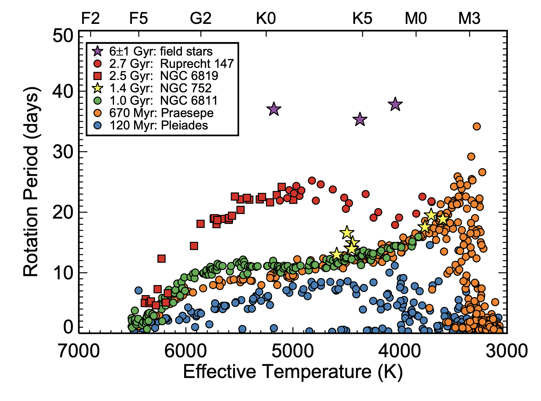
In the figure below from Curtis et al. (2020) (their Fig. 7), you can see observed distributions of rotation periods as a function of effective temperature (from Gaia DR2 colors) of stars in clusters and field stars of different ages. In this lab, we will make such a $T_{\mathrm{eff}}-P_{\mathrm{rot}}$ figure with MESA, using crowdsourcing.

Outline

A. Setting up your MESA work directory

• ~10 minutes
• Learn how to initialize a new MESA run directory from the default templates and understand the directory structure.

B. Setting up your MESA project inlist

• ~20 minutes
• Adjust the inlist files to define key input physics.

C. Setup pgplot and run the model

• ~25 minutes
• Use pgstar and log file outputs to live plot the evolution.

A: Setting up your MESA work directory

1. We will start from the default MESA work directory and build up our inlist. Make sure you have the MESA environment variables loaded. Start by copying over the default MESA work directory to some folder outside of MESA:

    cp -r $MESA_DIR/star/work work_lab1

Try to compile with ./mk. If everything compiled correctly (no errors), you should see a number of executables, namely clean, mk, re and rn when you type ls. The subdirectory src contains the run_star_extras.f90 file, which allows you to add additional physics and generate custom output. We will use this to add our own custom routine to apply magnetic braking via the option in the run_star_extras.f90 to provide an additional torque. For now, just simply replace the default run_star_extras.f90 file with the one of Lab 1 found here. You will learn about run_star_extras.f90 in the labs later in the week.

Everytime you change something to the run_star_extras.f90, you have to recompile to apply the changes. Make sure that you are in the work directory and type ./clean; ./mk to check if it compiles correctly.

The inlists contain all the input parameters for the MESA run. You will see inlist, inlist_pgstar and inlist_project.

The file inlist redirects MESA to the other two inlist files for all the real content, with inlist_project containing the input parameters and inlist_pgstar containing the parameters for the visuals MESA should produce during the run. Note that if you do not specifically set a parameter/control in the inlist, MESA assumes some default value that might not be optimal for your specific science case.

B: Setting up your MESA project inlist

2. We will now set the parameters/controls in the inlist_project. Open inlist_project with a text editor and replace the content with the inlist skeleton below. (There is a button to copy the entire block in the top right corner.) We first run a model without magnetic braking.

&star_job

      pause_before_terminate = .true. ! We pause the pgplot window when the run is finished.
      show_log_description_at_start = .true.

      ! pgstar

      ! pre main sequence

      ! initial rotation

      ! initial metal fractions



/ ! end of star_job namelist

&eos

/ ! end of eos namelist

&kap


/ ! end of kap namelist

&controls

      ! ZAMS limit

      ! uniform viscosity

      ! initial mass

      ! initial He and Z

      ! stopping criterion

      ! output

      ! atmosphere options

      ! Enable magnetic braking.
      use_other_torque    = .false.

/ ! end of controls namelist


&pgstar

! We set the pgstar controls in a separate inlist instead.

/ ! end of pgstar namelist

&colors

/ ! end of colors namelist

You will see different sections, indicated by for example

&star_job
/ ! end of star_job namelist

Let’s start with &controls. Pick a mass from the spreadsheet and set the initial mass equal to that value. If you have a less powerful machine, consider picking a higher mass. You can check the number of threads used for MESA with echo $OMP_NUM_THREADS, usually between 2 and 8.

initial_mass = 1d0

We want to run a model starting from the pre-main sequence up to the point when the hydrogen-mass fraction in the core ($X_{\mathrm{c}}$ ) is less than 0.01. First, in &star_job set

create_pre_main_sequence_model = .true.
pre_ms_T_c = 9.9d5 ! Initial central temperature.

Furthermore, in &controls set

xa_central_lower_limit_species(1) = 'h1'
xa_central_lower_limit(1) = 0.01

The initial composition of the star can be set by adding the following in &controls

initial_z = 0.0134
initial_y = 0.2485

The initial mixture (relative mass fractions of the metals) of the star can be set by adding the following in &star_job

   initial_zfracs = 6 ! AGSS09_zfracs

These three controls give us a star with a solar metallicity and metal fractions according to those measured for the Sun by Asplund et al. (2009).

$MESA_DIR/chem/public/chem_def.f90

Next, we will enable rotation. One option to do this, is by relaxing a non-rotating model to a specific uniform rotation frequency at the zero-age main sequence (ZAMS). We relax the ZAMS model in 15 steps to reach a velocity of $3.1416\cdot 10^{-5}$ rad/s, roughly 10 times the current surface rotation frequency of the Sun. Add in &star_job:

  new_omega =  3.1416d-5 ! 5000nHz
  set_near_zams_omega_steps = 15

We have to provide MESA with a working definition of the ZAMS, which we define here as the point where 95% of the total luminosity comes from nuclear reactions. In &controls, set

Lnuc_div_L_zams_limit = 0.95

We will enforce uniform rotation throughout the evolution. In MESA, the transport of angular momentum is done in a fully diffusive framework, where the efficiency is set by an effective viscosity. Diffusive transport wants to erase any gradient in the local rotation frequency. To enforce uniform rotation, we set the viscosity to a very high value, making the transport of angular momentum almost instantaneous. As mentioned before, if you do not set an inlist control yourself, MESA will assume a default value. First, have a look at the documentation to see what MESA does by default for the effective viscosity. The control that we need is called uniform_am_nu_non_rot.

Question: What is the default for the effective viscosity for angular momentum transport? Make sure it is enabled.

set_uniform_am_nu_non_rot = .true.
uniform_am_nu_non_rot = 1d20 ! in cm^2/s

In MESA, we have to make a choice on which opacity tables to use. MESA comes with several precomputed opacity tables for different sets of (X,Z), which are computed from monochromatic opacities, assuming a specific mixture. Since we want to be consistent with the Asplund et al. (2009) Solar mixture that we took, we use the appropriate opacity tables. Set the following controls in the &kap section.

!opacities with AGSS09 abundances
kap_file_prefix = 'OP_a09_nans_removed_by_hand'
kap_lowT_prefix = 'lowT_fa05_a09p'
kap_CO_prefix   = 'a09_co'

use_Type2_opacities = .false.

Type 2 opacities account for carbon and oxygen enhancement during and after He burning. We are not using those in this lab.

We also need to set the atmospheric boundary conditions. We are using a simple $T(\tau )$ relation for an Eddington grey atmosphere with a varying opacity in the atmosphere that is consistent with the local temperature and pressure. Add the following controls to &controls.

atm_option = 'T_tau'
atm_T_tau_relation = 'Eddington'
atm_T_tau_opacity = 'varying'

Pick a sensible name for the directory where all the output will be stored (in &controls), for example

log_directory = '1Msun_Z0p0134_Omega5000nHz_no_magnetic_braking'

To have MESA write out a row in the history file every time step, add the following in the same section.

history_interval = 1

Lastly, we want MESA to do live plotting of the evolution with pg_star. Set the following flag to true in &star_job:

pgstar_flag = .true.

Note that if you only change your inlists between runs, you do not need to recompile. Save the file and return to your work directory.

C: Running the models

3. Next, we will generate some custom plots during the run. We want to check that if there is no magnetic braking (no external torque), the total angular momentum of the star should be conserved. Replace inlist_pgstar with the one found here. Open inlist_pgstar with a text editor and add the following at the indicated place (although you can in principle place it anywhere).

Grid1_plot_name(7) = 'History_Track2'

History_Track2_title = 'total AM'
History_Track2_xname = 'log_star_age'
History_Track2_yname = 'log_total_angular_momentum'
History_Track2_xaxis_label = 'log_star_age'
History_Track2_yaxis_label = 'log_total_angular_momentum'

History_Track2_ymin = 47
History_Track2_ymax = 50

Save and return to your work directory.

History_Track2_xmin = <xmin>
History_Track2_xmax = <xmax>

4. We will now run our model (first without magnetic braking). In the work directory, run ./rn. You will see that after the relaxation phase MESA complains about the quantities that we want to plot in our custom window (ERROR: failed to find * in history data). This is because these quantities are not saved in the history file by default. You can stop the run prematurely with ctrl+C. The files that dictate what output should be saved can be found in

   $MESA_DIR/star/defaults/history_columns.list
   $MESA_DIR/star/defaults/profile_columns.list

   Copy the history_columns.list to your work directory and open it. Look for the quantities in the error messages and make sure they are uncommented (no ! in front). Also uncomment log_star_age and log_total_angular_momentum. Save and close the file, no need to recompile. If you rename your custom history_columns.list and profile_columns.list, you need to specify the names in &star_job.

   history_columns_file = 'custom_history_columns.list'
   profile_columns_file = 'custom_profile_columns.list'

   Let’s run the model again, ./rn. At some point, a window will show up.

   At the top left panel, you see the local angular rotation frequency (omega) as a function of the radial coordinate (in $R_{\odot }$ ). Since we enforce uniform rotation, you should see a flat line. Next to this panel, you see the local chemical diffusion coefficient (log D) as a function of the mass coordinate (m) in Solar mass units. The blue regions are convective regions and have such high diffusion coefficients that the material is instantaneously mixed within the convective zones. Since we do not include any rotational mixing, the other colors in the legend should not show up.

   If the pgplot window does not fit your screen properly, you can change the following controls in inlist_pgstar.

   Grid1_win_width = <value>
   Grid1_win_aspect_ratio = <value>

Question: Have a look at our custom plot showing the total angular momentum over time. Is it indeed conserved (after relaxation)? (You may stop the run if you are convinced.)

5. Now we will turn on magnetic braking. The quantity that we need for this is the change of the total angular momentum $J$ over time. We make a distinction between the regime where the magnetic field strength is saturated and when it is growing. The regime that we are in is defined by the convective Rossby number, the ratio of the (surface) rotation period over the convective turnover time, $\mathrm{Ro}=P_{\mathrm{rot}}/{\tau }_{\mathrm{conv}}$ . The Rossby number is a dimensionless parameter in fluid dynamics representing the ratio of inertial forces to Coriolis forces in a rotating fluid. It has been shown to correlate strongly with stellar magnetic activity (Noyes et al. 1984).

We adopt a $\mathrm{d}J/\mathrm{d}t$ prescription that appears to reproduce many observed cluster properties (see Fig. 2 of Chiti et al. 2024), following the work of Kawaler (1988) and van Saders & Pinsonneault (2013). If $\mathrm{Ro}<\mathrm{R}{\mathrm{o}}_{\mathrm{sat}}$ (saturated),

If $\mathrm{Ro}>\mathrm{R}{\mathrm{o}}_{\mathrm{sat}}$ (unsaturated),

where

Furthermore, $K$ , ${\tau }_{\mathrm{conv},\odot }$ and ${\mathrm{\Omega }}_{\mathrm{sat}}$ are constants that need to be calibrated.

We do not expect significant magnetic braking when the Rossby number exceeds a critical value (Saunders et al. 2024), which we take as,

To enable the magnetic braking run_star_extras routine, we set the following flag in &controls equal to True.

! Enable magnetic braking.
use_other_torque    = .true.

This enables the custom magnetic braking routine in the run_star_extras.f90. Change the name for the output log directory to save this run in a new folder. Check the evolution of the total angular momentum again. Do you now observe any angular momentum loss? Hit Enter once you have finished inspecting the plots.

Task: Note down the effective temperature and rotation period at the 5 different points in age displayed at the end of the run in the spreadsheet. If your star does not reach the older ages, leave those blank.

Bonus question: How is the rotational evolution affected by the initial rotation velocity (new_omega)?

&star_job

      pause_before_terminate = .true.
      show_log_description_at_start = .true.

      ! pgstar

      pgstar_flag = .true.

      ! pre main sequence

      create_pre_main_sequence_model = .true.
      pre_ms_T_c = 9.9d5 ! Initial central temperature.

      ! initial rotation

      new_omega =  3.1416d-5 ! 5000nHz
      set_near_zams_omega_steps = 15

      ! initial metal fractions

      initial_zfracs = 6 ! AGSS09_zfracs

/ ! end of star_job namelist

&eos

/ ! end of eos namelist

&kap

      ! opacities with AGSS09 abundances
      kap_file_prefix = 'OP_a09_nans_removed_by_hand'
      kap_lowT_prefix = 'lowT_fa05_a09p'
      kap_CO_prefix   = 'a09_co'

      use_Type2_opacities = .false.

/ ! end of kap namelist

&controls

      ! ZAMS limit
      Lnuc_div_L_zams_limit = 0.95

      ! uniform viscosity
      set_uniform_am_nu_non_rot = .true.
      uniform_am_nu_non_rot = 1d20 ! in cm^2/s

      ! initial mass
      initial_mass = 1.2d0

      ! initial He and Z
      initial_z = 0.0134
      initial_y = 0.2485

      ! stopping criterion
      xa_central_lower_limit_species(1) = 'h1'
      xa_central_lower_limit(1) = 0.01

      ! output
      log_directory = '1p2Msun_Z0p0134_Omega5000nHz_magnetic_braking_test'
      history_interval = 1

      ! atmosphere options
      atm_option = 'T_tau'
      atm_T_tau_relation = 'Eddington'
      atm_T_tau_opacity = 'varying'

      ! Enable magnetic braking.
      use_other_torque    = .true.

/ ! end of controls namelist

&pgstar

! We set the pgstar controls in a separate inlist instead.

/ ! end of pgstar namelist

&colors

/ ! end of colors namelist