Lab 1: Give and Take

Overview

Massive stars $(M\gtrsim 8M_{\odot })$ are overwhelmingly part of binary (or even higher order) systems. See this figure from Offner et al. (2023)¹ that compiles data from many multiplicity studies: When such stars evolve, they engage in mass-transfer events, which create a whole host of astrophysical phenomena that cannot not be understood with single-star evolution. One of the best examples are X-ray binaries, where a dense neutron star (or black hole) is accreting material from its companion star: Artist impression of a mass-transferring X-ray binary. The disk of the accretor becomes very hot and emits X rays. Credit: ESO/L. Calçada/M.Kornmesser.

This lab will introduce you to the inner workings of MESA/binary, and give you an understanding of how massive stars exchange mass.

Anatomy of a binary

Simulating single stars is fun, but simulating binary stars is even more fun. MESA can do this by separately solving the equations of stellar structure on both objects, and potentially link them by invoking interaction routines.

Imagine two rows of boxes, representing the stars. Each box is filled with the properties of the interiors ($T,\rho ,r,L,X$ ), varying from the cores to the surfaces. MESA/star is in charge of evolving those two rows of boxes by advancing the time by $\Delta t$ , and solving the stellar-structure equations, keeping in mind all of the required microphysics (nuclear nets, eos, opacities, mixing, etc…). A binary star, however, is more than just its two components. The two objects are orbiting each other, which requires 4 variables to fully specify (we do not care about the orbit’s orientation to a potential observer). We choose them to be the masses of the objects, the orbit’s angular momentum, and its eccentricity.

Each variable has an associated evolution equation, e.g.:

MESA/binary’s job is to carefully track the orbital quantities, i.e., compute the values $d{M}_1/dt$ (which it passes on to MESA/star who actually performs the mass change and the associated remeshing of the model), $dJ/dt,$ etc… MESA/binary also needs to check that the resulting state of the binary star is “acceptable.” Consider the following two example cases:

1. If ${\dot{M}}_{1,\mathrm{transfer}}=0,$ and neither star overflows its respective Roche Lobe, we are good, as this fulfills the requirements for a non-interacting binary.
2. On the other hand, if it turns out that the evolution of the donor (as reported by MESA/star) is such that its radius is larger than its Roche Lobe radius, the roche_lobe scheme of mass transfer is violated! We have to redo the step with a higher mass-transfer rate, so that (hopefully) this reduces the radius of the donor star to just within the Roche Lobe radius. MESA/binary will iterate this process until it finds a mass-transfer rate that leaves the donor just inside its Roche Lobe. Note that the Ritter or Kolb schemes work very differently: There, MESA compares the mass-transfer rate assumed at the start of the step with the mass-transfer rate computed from the physical properties at the end of the evolutionary step, and only accepts the step if those agree to within a set tolerance. Both these schemes, where properties at the end of the step are compared to certain criteria, are called implicit determinations of the mass-transfer rate, and improves stability of the evolutionary calculations.

How to do binaries in MESA

MESA/binary has its own set of controls to setup in the initial condition of the binary, manage the physics of mass transfer and tides, and it has its own set of timestep controls (for example to not let the mass-transfer rate change too quickly from step to step).

All of these control options and their defaults are listed on the docs under Reference and Defaults > Binary defaults.

The actual running of a binary simulation is similar to that of a single star:

1. use a work directory based on the $MESA_DIR/binary/work directory (you’ll notice that the contents of the make/ and src/ folders are slightly different so trying a binary run with the default star/work direction would not work.)
2. do ./mk to compile the run_binary_extras routines (even if they’re empty/do nothing)
3. do ./rn to start the simulation.

With the most basic concepts of MESA/binary out of the way, let us continue by exploring the science of massive binary stars and their interactions.

Mass transfer cases

The common thread through the series of labs today is how we think gravitational wave (GW) mergers are produced. Since September of 2015, GW mergers involving neutron stars and black holes are being detected with the LIGO, VIRGO, and KAGRA detectors (referred to as LVK). However, we aren’t yet fully certain how those black holes are formed. Is it through dynamical interactions in clusters that they get paired up? Maybe they come from the very first pop-III stars (those are stars born very early in the universe, lacking basically any metals; $Z\approx 0$ ) that makes them so massive?

The scenario we’re exploring here is called isolated binary evolution. This assumes we start with two (massive) stars born together in a binary. As they evolve, go supernova, and leave behind two compact objects, we hope that they are close enough to merge in a time less than the age of the universe (called a Hubble time ${\tau }_H=H_0^{-1}\approx 14.5\mathrm{Gyr})$ .

Let’s zoom in on the first part of binary evolution: Two stars which undergo mass transfer:

When stars evolve, they (generally) become bigger over time. As soon as the most massive star evolves to fill its Roche Lobe (RL), mass transfer will ensue, called Roche Lobe overflow, or RLOF. Depending on the evolutionary stage of the donor, we distinguish different mass transfer cases. When the donor is still (core) hydrogen burning, we speak of case A mass transfer, while when it is core-helium burning, we have case B, and there’s even case C for mass transfer post-core-helium exhaustion.

The main parameter controlling when mass transfer will occur is the initial orbital period. For massive stars, the rule of thumb is that case A occurs (roughly) for initial periods under 10 days, and case B occurs between 10 and 1000 days (with case C at a small interval of even larger periods).

Run 1: Case A evolution: Tidal domination

When interaction occurs during the main sequence, the initial period of the system must be small, because the stars are compact (relative to post-main-sequence (super-)giants). We therefore expect that the tidal interaction between stars that orbit each other so tightly to be very strong. Let’s see what this does to the rotation rate of the stars in this system.

Look and search through the inlist defaults to set up the following:

• Set the initial period to 3 days.
• Enable the effects of tidal synchronization. Then, set the sync_type of both stars’ tidal prescription to Orb_period.
• Load the initial stellar models, zams35.mod and zams25.mod, in the &star_job sections of inlist1 and inlist2, respectively (ZAMS = zero-age main sequence = star at birth).

   ! initial conditions
   initial_period_in_days = 3d0

   ! tidal sync setting
   do_tidal_sync = .true.
   sync_type_1 = "Orb_period"
   sync_type_2 = "Orb_period"

   load_model_filename = 'zams35.mod'  ! select correct model for star 1!

   load_model_filename = 'zams25.mod'  ! select correct model for star 2!

Start the MESA run with ./mk and ./rn, just as you’d do for single-star evolution!

A (rather busy) pgbinary plot like this will pop up: As indicated above, it has three large sections, one for the pgstar info of either star (using the pgbinary plot type Star), and the third column for information inherent to the binary itself. The info in the Star plots is controlled by what is read into the &pgstar inlist section of the respective stars (inlist1 and inlist2, but in this case they both point to the same thing, inlist_pgstar). The star plots show (among others) the composition & mixing profiles, HRD, radius evolution, and some textual info at the bottom, while the binary column shows the orbital configuration, the radii compared to the Roche Lobe radii, orbital period, and mass-transfer rate.

During the run, watch the following quantities:

1. Can you find the mass-transfer efficiency (and what does this mean?) What is the typical mass-transfer rate, ${\dot{M}}_{\mathrm{trans}}$ , of this binary system? Is it constant over time (or model number)? Can you identify multiple distinct mass-transfer phases based on the value of ${\dot{M}}_{\mathrm{trans}}$ ?

   Hints

   Look at lg_mtransfer_rate and its associated graph. Also watch the eff_xfer_fraction (the “effective transfer fraction”) number. Don’t be alarmed if the xfer_fraction is negative when no mass transfer is happening, that is because it is naively calculated as eff_xfer_fraction = -dot_M2 / dot_M1, which contains contributions from the stellar winds.

   Result

   Mass transfer efficiency is the ratio of mass accreted over the amount donated. You can see two distinct phases of mass transfer in the lg_mtransfer_rate plot; case A and later case AB when the primary exhausts hydrogen and tries to become a giant. The first mass-transfer phase can be further split in 2: a high mass-transfer rate fast case A followed by a more mellow slow case A where the mass transfer rate is a couple of orders of magnitude lower.

2. Are the stars in thermal equilibrium during any of the mass-transfer phases? If not, how does this manifest?

   Hints

   Take a look at the luminosity profiles; thermal equilibrium is defined as $dL/dm={ϵ}_{\mathrm{nuc}}$ . Where is nuclear burning occurring? You can find out by looking at the stars’ profiles. Also, compare the numbers for the kh_timescale and the mdot_timescale in the text summary of both stars.

   Result

   You should see that neither star satisfies it during rapid mass-transfer phases. The donor’s luminosity profile dips significantly in the envelope, so that $dL/dm\ne 0$ , but we have that ${ϵ}_{\mathrm{nuc}}=0$ as no burning takes place there. The accretor is slightly more luminous than its nuclear luminosity, due to the accretion energy it gains. You should see that neither star satisfies thermal equilibrium during rapid mass-transfer phases. In the slow case A phase, thermal equilibrium is nearly satisfied, as the thermal timescale of the stars is much shorter than the mass-transfer timescale.

3. Rotation rates: Do the stars spin up or down significantly during mass-transfer events?

   Hints

   Look at the omega_div_omega_crit profiles of either star.

   Result

   The stars rotate appreciably, at around 50% of critical. But importantly, the tidal forces prevent the stars from rotating close (i.e., >95%) to their critical velocity!

4. How does the orbital period evolve during the mass-transfer events?

   Result

   The orbital period will first decrease somewhat, until the mass ratio ($M_2/M_1$ ) has reached a value of roughly 1. From that point on, the period will increase since mass transfer is happening from a lower to a higher mass star

5. At the end of the run, what is the state of both of the stars? Is the secondary star significantly evolved (check the abundance profiles!)? Are their surface conditions different? Note down the carbon-core mass of the primary, and surface rotation rate of the accretor, you might need these numbers later.

   Result

   The donor star looks very different from the accretor. The donor is a hot and compact helium-rich star that has almost depleted helium in its core. The accretor on the other hand is a relatively normal main-sequence star. The donor’s CO core mass should be roughly $13.6M_{\odot }$ , and the accretors surface rotation rate is approximately 15% of the critical velocity.

Run 2: Case B evolution: You spin me ‘round!

Case B mass transfer occurs in binaries that get born slightly wider. The wider the binary, the weaker the tidal forces (they scale with the separation to the power 6!). In this run therefore, we will simulate weaker tides.

Setup:

• Edit inlist_project so that this system has an initial period of 20 days.
• Change the tides prescription from Orb_period to Hut_rad. The prescription of Hut (1981)² is a physically motivated computation of how tides operate in the radiative envelopes of massive stars.

Run the simulation, and watch as the primary star first exhausts hydrogen before a phase of mass transfer starts. Tasks for this run:

1. Use pgbinary to plot the efficiency of mass transfer, and see how it evolves over the mass-transfer event

   Hint

   Either expand the History_panels1 in &pgbinary by one panel, and plot the eff_xfer_fraction there, or add it to an already existing panel if the _other_yaxis is still free.

   Solution

   History_panels1_other_yaxis_name(3) = 'eff_xfer_fraction'
   History_panels1_other_ymin(3) = -1
   History_panels1_other_ymax(3) = 2

   or

   History_panels1_num_panels = 4
   ...
   History_panels1_yaxis_name(4) = 'eff_xfer_fraction'
   History_panels1_ymin(4) = -1
   History_panels1_ymax(4) = 2

2. How does MESA handle the accretion onto the secondary? Is some condition met that prevents the star from accreting more?

   Hint

   The terminal output should write things like: fix w > w_crit: change mdot and redo. Why would MESA write this?

   Explanation

   MESA is changing the accretion rate of the secondary so that its rotation rate remains below ${\Omega }_{\mathrm{crit}}$ . The donor is supplying a certain amount of mass per unit time, and MESA needs to figure out how much of it to accept to keep the secondary star from spinning so fast that it starts tearing itself apart (ejecting the rest as a fast wind).

3. Watch the rotation rate of the accretor closely.

   Hint

   Do you see anything peculiar about the profile of omega_div_omega_crit?

   Hang on now?!

   What is this? $\Omega /{\Omega }_{\mathrm{crit}}>1$ ? How can this be? I thought the mass-accretion rate made sure the star spins below critical?

   The plot thickens…

   MESA is doing more than just comparing the angular velocities of the surface cell alone. Take a look at lines 845-848 of ‘$MESA_DIR/star/private/evolve.f90`:

   w_div_w_crit_prev = w_div_w_crit
   ! check the new w_div_w_crit to make sure not too large
   call set_surf_avg_rotation_info(s)
   w_div_w_crit = s% w_div_w_crit_avg_surf

   What does this set_surf_avg_rotation_info routine do? Remember you can (recursively) search through files in UNIX with:

   $MESA_DIR/star/private $> grep -rin "set_surf_avg_rotation_info"

   The discrepancy revealed!

   MESA computes a mass-averaged value of the rotation rate from cells with optical depth surf_avg_tau_min to surf_avg_tau, which is 1 to 100 by default. Since most of the mass is at optical depth 100, you can effectively read off where the $\tau =100$ surface lies; it’s where omega_div_omega_crit = 1. This also makes it possible that the (very tenous) outer layers spin “faster” than critical. This doesn’t necessarily mean this is a bad approximation, however, as the stellar wind will quickly blow away these layers once mass transfer stops.

4. Establish what the tidal synchronization timescale is of the stars, and plot it. Compare it to the mass-transfer timescale (especially for the accretor during mass transfer).

   Hint

   Scour the list that binary defines as default history columns, in your binary_history_columns.list. Uncomment the entries you find there, and rerun your model to make sure you now have the output. You can use pgbinary panels to plot these values on the fly. The mass-transfer timescale is already printed in the &pgstar text, as mdot_timescale.

   Solution

   Spot the following lines:

       lg_t_sync_1 ! log10 synchronization timescale for star 1 in years
       lg_t_sync_2 ! log10 synchronization timescale for star 2 in years

   so we can plot in &pgbinary:

       History_panels1_num_panels = 4
       ...
       History_panels1_yaxis_name(4) = 'lg_t_sync_1'
       History_panels1_other_yaxis_name(4) = 'lg_t_sync_2'

Run 3: Case B evolution: You spin me ‘round?

It is good to realize that since we model everything in 1D, our assumptions about how much mass transfer spins up the accretor, and how or where mass is lost is unavoidably based on some assumptions. There is no consensus on how (non)-conservative mass transfer should or would be for a particular binary system governed by a particular set of input physics.

Above, we modeled accretion happening in a system with weak tides, and that turned out to spin up the accretor star very rapidly, causing very inefficient mass transfer (not much of the donated mass ended up being accreted by the companion). Many observed systems, however, indicate conservative mass transfer is preferred.

Typically, we characterize mass-transfer efficiency, $ϵ$ , using 4 parameters: $\alpha$ , $\beta$ , $\gamma$ , and $\delta$ . The parameters control whether we consider the non-accreted mass to be lost near the donor ($\alpha$ ), near the accretor ($\beta$ ), or through a circumbinary disk ($\delta$ , and the disk has a dimensionless radius of $\gamma =\sqrt{R/a}$ ). We then define:

If $ϵ=1$ , mass transfer is conservative, while $ϵ=0$ means mass transfer is fully non-conservative. In this run, we’ll set up the physics to model this kind of accretion, and see what consequences this has on the structure of the stars and the evolution of the orbit.

When accreting, only the surface layers tend to spin up, while the deeper layers below still rotate quite slowly. This is because angular-momentum transport down to the core is not that efficient (we’ll see more of this in the next lab). In this run, we’ll use our god-like powers as MESA users to crank up the efficiency of angular-momentum transport artificially.

Setup:

• Set the tidal prescription back to Orb_period for both stars.
• Search for the mass-transfer efficiency parameters in the reference. We want to simulate a fraction of the mass getting ejected from the vicinity of the accretor.
• We want to artifically induce very efficient internal angular-momentum transport in both stars. You can do this by setting set_uniform_am_nu_non_rot = .true. and picking a very high number for uniform_am_nu_non_rot. With this setting we simulate a non-rotational angular-momentum diffusion process. Note that this is a stellar process, not a binary one, so check the reference in which inlist section this control belongs.
• Since we will not hit the rotational limit as much, tighten the implicit wind calculation tolerance, adjusting surf_omega_div_omega_crit_tol to 1d-2.
• Lastly, pick a secondary mass, initial period, and $\beta$ from the Google Sheet, and run the simulation.
  Solutions

  An example of &binary_controls would be:

     ! initial conditions
     initial_period_in_days = 50d0
  
     ! tidal sync setting
     do_tidal_sync = .true.
     sync_type_1 = "Orb_period"
     sync_type_2 = "Orb_period"
  
     ! constant efficiency
     mass_transfer_beta = 5d-1

  and inlist2 should load the correct mass:

     load_saved_model = .true.
     load_model_filename = 'zams27.5.mod'  ! select correct model for star 2!

  &controls of inlist_star should contain:

     surf_omega_div_omega_crit_tol = 1d-2
  
     set_uniform_am_nu_non_rot = .true.
     uniform_am_nu_non_rot = 1d20

  or any higher number for the diffusion coefficient.

Take note of the following during the run:

• How does the accretor respond to the transferred mass? Does it spin up? Why (not)? Does the mass-transfer efficiency agree with your chosen $\beta$ ? Are there multiple mass-transfer phases?

  Solution

  Your star’s spin should correlate with its size. The star will puff up when accepting a lot of mass, sometimes leading to a short contact phase depending on the chosen parameters. The efficiency should closely agree to $1-\beta$ . If there is a slower case B mass transfer, efficiency can be lower because the stellar wind starts to take a signicant fraction of the mass-loss budget.

• Compare the synchronization timescale to what you had in the previous run. See any difference? Does this explain the rotation rate of the secondary?

  Solution

  The synchronization timescale is of order $10^{-1}\mathrm{yr}$ , which is way shorter than the typical integration step (see the log_dt graph). Hence the star is quickly synchronized to the orbital period.

• Record the final masses and period into the Google Sheet. Compare with the value that Soberman et al. (1997)³ predicts from angular-momentum-balance arguments (automatically calculated in column K). How would you explain any discrepancy between Soberman’s and your obtained number?

  Solution

  Soberman’s calculation does not take gravitational radiation, spin-orbit coupling (through tides), and wind-mass loss into account. These are all extra terms one would have to take into account when calculating the final period.

Conclusions

These MESA/binary runs should have given you a feel for how one goes about setting up two stars in a binary orbit, what kinds of physics one can modify to simulate different modes of mass transfer, and how this affects the rotation rate of the accretor. In the end, we have created a Wolf-Rayet (WR) binary:

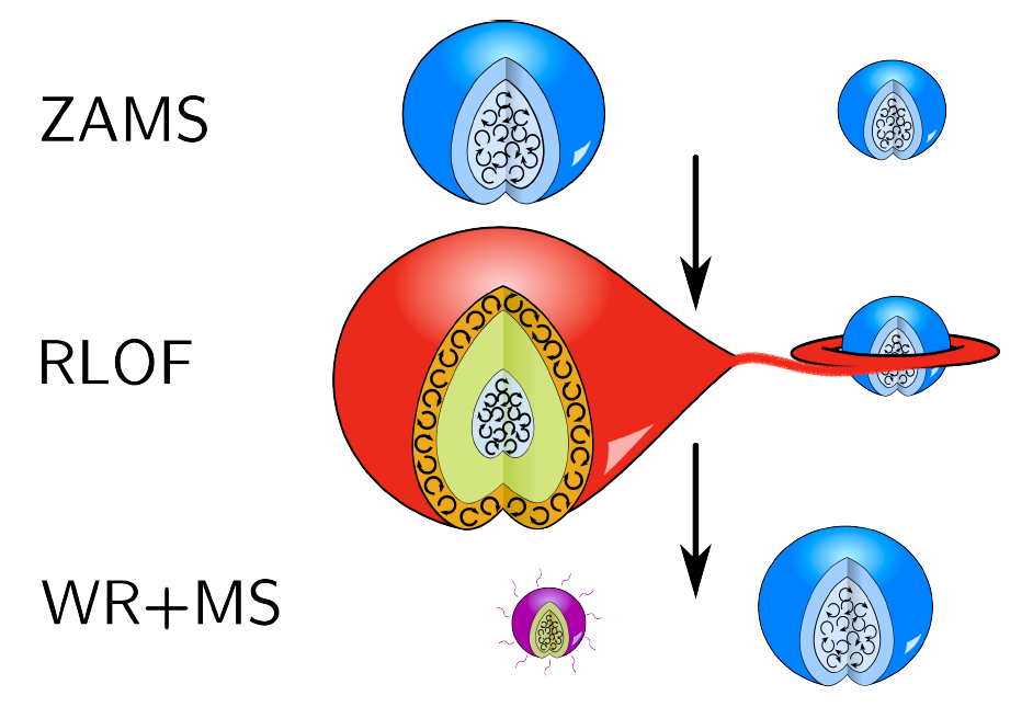
and the once less massive star is now the more massive star. WR stars are typically helium rich (because their hydrogen layers have been removed; the exception here are the very massive WNh-type WRs), and they launch a very thick stellar wind. In spectroscopic observations such systems reveal themselves with strong and broad emission lines. This system will continue to evolve, and we’ll pick up this thread again in Lab 3 this afternoon.

Final models and inlist sets

If you were short on time, below you can find:

• the final models of Run 1 (case A), as well as of Run 3 with $M_2=25M_{\odot }$ , $\beta =0$ , and $p_i=20\mathrm{d}$ (case B).
• final inlists after Run 3.

$\star$ Bonus exercices $\star$

If you have extra time after Lab 1, take a look at these bonus exercises to enhance your skills working with MESA/binary.

Extra history columns

MESA/binary produces a separate history file, appropriately named binary_history.data, which contains information on the state of the binary. For this exercise, implement the “observational mass ratio” as an extra binary history column (for any of the runs you did in the main lab). This is the ratio of the less massive to the more massive star. As an observer measuring masses of stars, you have no a priori information of what the “primary” is, and so it is customary to define $q\equiv M_{\mathrm{low}}/M_{\mathrm{high}}<1$ , rather than $q=M_2/M_1$ , which can flip from below one to above as the binary evolves.

integer function how_many_extra_binary_history_columns(binary_id)
    use binary_def, only: binary_info
    integer, intent(in) :: binary_id
    how_many_extra_binary_history_columns = 1
end function how_many_extra_binary_history_columns

subroutine data_for_extra_binary_history_columns(binary_id, n, names, vals, ierr)
    use const_def, only: dp
    type (binary_info), pointer :: b
    integer, intent(in) :: binary_id
    integer, intent(in) :: n
    character (len=maxlen_binary_history_column_name) :: names(n)
    real(dp) :: vals(n)
    integer, intent(out) :: ierr
    real(dp) :: beta
    ierr = 0
    call binary_ptr(binary_id, b, ierr)
    if (ierr /= 0) then
        write(*,*) 'failed in binary_ptr'
        return
    end if
    names(1) = 'obs_mass_ratio'
    if (b% m(1) > b% m(2)) then
        vals(1) = b% m(2) / b% m(1)
    else
        vals(1) = b% m(1) / b% m(2)
    end if

end subroutine data_for_extra_binary_history_columns

Modeling the sdO binary $\varphi$ Persei

$\varphi$ Persei is a lower mass binary containing a subdwarf (sdO) and a B2 main-sequence star. From its orbital period, we infer it must have undergone case B mass transfer when the now-subdwarf star overflowed its Roche Lobe. While not being a binary black-hole progenitor, its evolution is still very interesting to model. In the future it’ll likely undergo a common envelope phase (see also lab 3):

• If this succesfully ejects the envelope of the giant star, a double white dwarf binary will be created (which may be observable with space-based GW detectors such as LISA),
• If unsuccesful in ejecting the envelope, the stars will merge an exotic late core-collapse supernova can occur (in a system where neither star individually would go supernova; this shows that binary evolution can drastically change the outcome of stellar evolution).

In this exercise, you’ll try to recreate the history of $\varphi$ Per using MESA.

Image of $\varphi$ Persei. Credit: David Ritter, license: CC BY-SA 4.0.

$\varphi$ Persei’s observed properties are:

You won’t have time to compute a full grid of models for different sets of initial conditions, so you’ll have to make clever choices for the initial parameters of this system. First, try to figure out what stellar masses you want to start with. From observation we know that the sdO is essentially the helium core of a star that lost its entire hydrogen envelope. Knowing that this core is formed from roughly 20% of the initial mass of the star at ZAMS, you can get an estimate of what $M_{1,\mathrm{init}}$ has to be.

You then also know what amount of mass will be lost from the donor, which will transfer to the secondary, and be available to be accreted. Calculate the amount of mass accepted by the accretor assuming an efficiency $ϵ=1-\beta$ . Of course, after the mass-transfer event, we should end up with $M_2=9.6M_{\odot }$ of mass, so choose appropriate values for $M_{2,\mathrm{init}}$ and $\beta$ to make the math work. Remember that $M_{2,\mathrm{init}}<M_{1,\mathrm{init}}$ because otherwise the secondary starts mass transferring first!

Settings to change from the Run 3 setup:

• Disable the step overshoot we use for (very) massive stars. The remaining exponential overshoot is plenty for this example.
• Set the appropriate ZAMS models. Download this grid as the set of starting models, and move it to $MESA_DIR/data/star_data/zams_models/. Don’t use the load_saved_model functionality, but instead set, in &controls of inlist_star:

zams_filename = 'zams_z142m2_y2703.data'
initial_z = 0.0142d0
initial_y = 0.2703d0

and set your chosen initial masses and initial period in &binary_controls.

See if you can get both masses to within $0.1M_{\odot }$ and the final period to within 5% of the observed values. If you’d like, share your solution to the Google Sheet in the right-most tab.

Things to consider after this exercise:

• Convince yourself that the mass transfer in this system can’t have been very non-conservative.
• What would’ve had to be different about the observed properties for a non-conservative scenario to work?
• If you really want to nail down the sdO mass, but you couldn’t change the initial mass, what parameter(s) would you change? Try it!

References