Lab 2: Stellar Swinging
Overview
In the previous lab, we have seen how stellar expansion leads to mass transfer, which affects their mass, radius, and orbital separation.
However, rapid rotation can fundamentally change this picture. Rotation can have dramatic effects on the mass-radius relation, and as a consequence on the occurrence of mass transfer. In Lab 2, we will look at the effect of rapid rotation on the structure of stars and their black hole (BH) products. Along the way, we will also learn how to add a brand new history column to our output.
Move 1: introduction to chemically homogeneous evolution

Very close stars want to face each other.
Rapidly rotating stars become rotationally deformed (oblate), which prevents them from being simultaneously in hydrostatic and thermal equilibrium (the von Zeipel paradox). To resolve this, large-scale currents develop throughout the radiative envelope: material sinks toward the center at the equator and rises to the surface at the poles. These Eddington-Sweet (ES) circulations 12, or meridional circulations, mix hydrogen from the outer envelope into the convective core, causing the star to evolve as a single well-mixed entity. We call this chemically homogeneous evolution (CHE).
The ES timescale (i.e., how long a circulation takes to transport a mass element all the way from core to surface) is roughly
where is the star’s thermal timescale, is its angular rotation speed (assuming rigid body rotation), and is its critical (at which the centrifugal force equals gravity on the surface). For ES circulations to be effective, we need a short ES timescale, and CHE thus requires the star to maintain near-critical rotation throughout the MS. This can be achieved in a very tight binary where tidal synchronization keeps the star spinning rapidly for the duration of the MS.
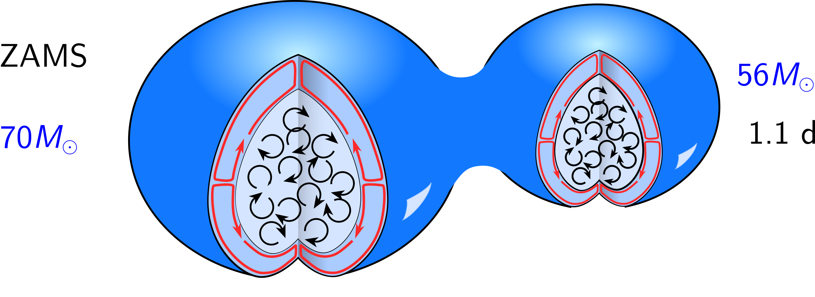
Schematic of a CHE binary at Zero-Age Main Sequence (ZAMS). This represents a case of a CHE binary as a contact binary, which we are not modeling in this lab.
Because CHE stars lack a core-envelope structure, they never develop the expanding envelope that would otherwise drive mass transfer. Instead, they remain compact during the MS and further contract afterwards. In the HR diagram, CHE stars evolve to the left (hotter temperatures), rather than expanding to the right as cool RSGs. As they evolve, they become progressively hydrogen-free, and you are left with a bare He star and potentially a Wolf-Rayet star.
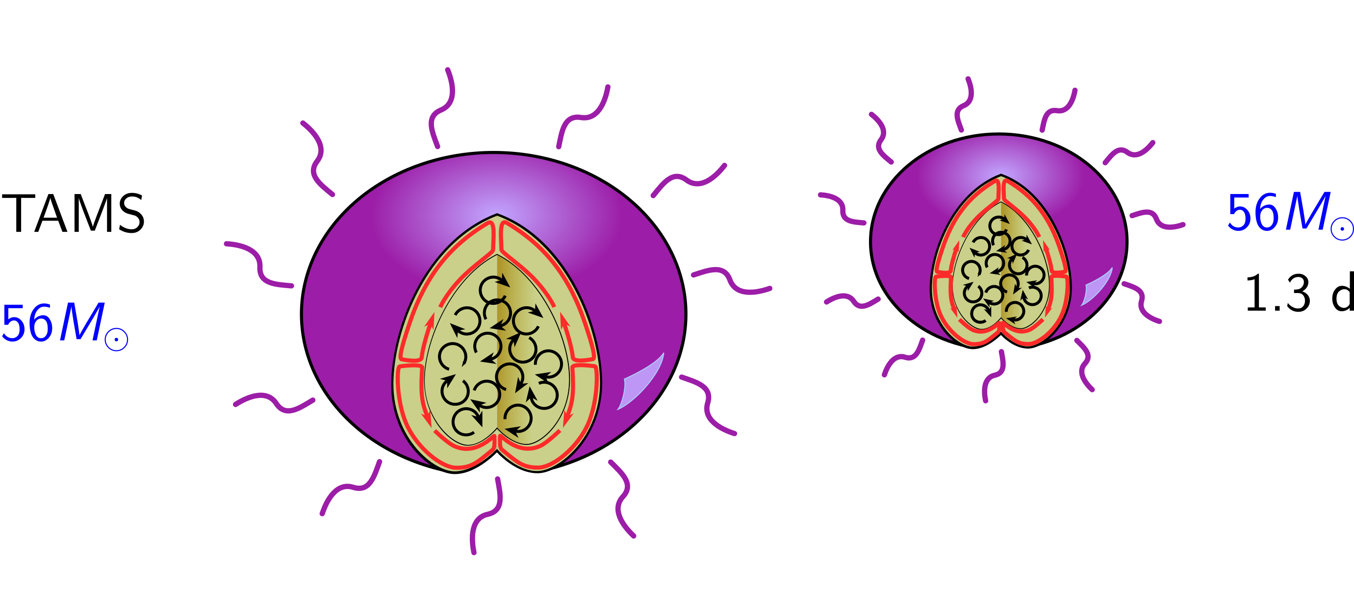
Schematic of a CHE binary at Terminal Age Main-Sequence (TAMS).
Move 2: starting in close position, or CHE stars in the MS

CHE stars avoid stepping on each other's foot! (or Roche lobe)
Since the timescale of ES circulation depends primarily on stellar mass and rotation rate, let’s place our massive stars in short-period binaries where tides maintain rapid rotation and see what combinations of mass and orbital period produce CHE.
Tip
When setting up inlists, you can find all options for star and binary either within $MESA_DIR/star/defaults and $MESA_DIR/binary/defaults, respectively; or in the References and Defaults section of the online documentation. The content is the same.
Move 2.1: set up your work folder
To get started, set up a work folder for Lab 2, then download to it the initial_model folder from here and unzip it. Do the same for the binary_template folder from here. The initial_model contains a basic single star setup to generate our Zero-Age Main Sequence (ZAMS) models. In binary_template, the inlists contain most of the settings for our runs, and the .list files necessary output. The src/run_star_extras.f90 contains a custom implementation of stellar winds geared towards CHE stars. We will later go back to the extras file.
Downloading and unzipping
wget <url> or curl -O <url>. Files can be directly unzipped in the terminal with unzip filename.zip. unzip is available through most default package managers such as apt, dnf or brew — e.g., call sudo apt install unzip.Move 2.2: produce your ZAMS model
With your work folder setup, choose one of the following mass-period pairs for your stars, which reliably lead to CHE, and which you will carry through to the end of the lab. More massive stars take longer to run, so pick based on how your computer performed in previous labs!
| 40 | 1.00 |
| 70 | 1.20 |
| 100 | 1.50 |
| 300 | 2.20 |
You will first generate the ZAMS model for your binary. Go into initial_model and add the mass setting in inlist_project, then clean (./clean), compile (./mk) and run (./rn). Once the run is complete (it should take only a few seconds), copy the produced zams.mod to the binary_template folder.
Solution
Add to inlist_project,
&controls
    initial_mass = ! your mass
Move 2.3: adapt binary_template to CHE binaries
CHE stars in binaries are amenable to being treated as twins because they are generally expected to have nearly equal masses (when tides are strongest) and suffer near net-zero mass transfer (being compact). This allows us to solve only the primary’s structure; we’ll tell MESA to treat the secondary as if it were identical to the primary. This cuts our runtime in half!
We will manually adapt the setup in binary_template to evolve our stars as twins. MESA already has a setting for this, which you will be able to find in the inlist defaults.
Warning
Even when you set the stars to be treated as twins, you must explicitly set the secondary to have the same mass as the primary.
The inlist_star file is already set up for a CHE star and to load zams.mod as a starting model. In inlist_project,
- Point the primary to
inlist_star, set the secondary to have the same starting mass as the primary, and set the initial orbital period.Solution
Add
&binary_job
   inlist_names(1) = 'inlist_star'
and
&binary_controls m2 = ! your chosen mass initial_period_in_days = ! your chosen period - Tell MESA to set the stars as twins in the initial model.
Solution
Add
&binary_job
   change_initial_model_twins_flag = .true.
   new_model_twins_flag = .true.
Move 2.4: run your CHE binary!
In binary_template, launch your new binary with ./clean; ./mk; ./rn. As your model is running, work through the following tasks:
Watch the pgplot window, in particular the HR diagram and the diffusion coefficient plot. Is your star evolving CHE? How can you tell? Look at the different diffusion coefficients: what do they represent, and how do different mixing modes contribute to mixing from center to surface?
Solution
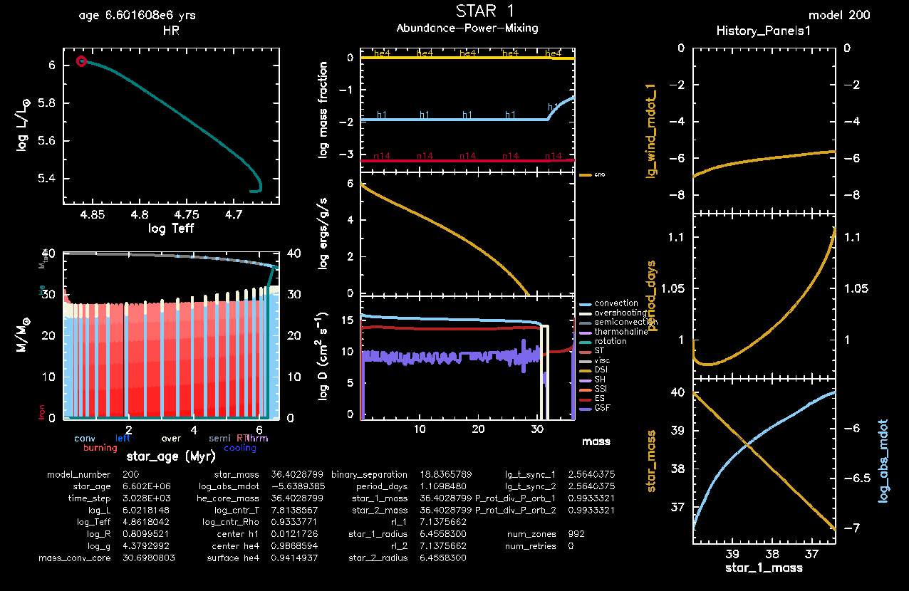 If your star is going CHE, it should move blue-wards in the HR diagram (to the high temperatures, to the left) for almost the entire MS, indicating very little to no expansion. While the example above is for the
case specifically, this blue-wards trend is present for CHE stars of any mass. If it starts moving red-wards, MESA will stop the run very soon due to it not going CHE.
If your star is going CHE, it should move blue-wards in the HR diagram (to the high temperatures, to the left) for almost the entire MS, indicating very little to no expansion. While the example above is for the
case specifically, this blue-wards trend is present for CHE stars of any mass. If it starts moving red-wards, MESA will stop the run very soon due to it not going CHE.In the diffusion panel, you should be able to find the convective core (dominated by ) and the overshooting layer above it ( ). Everything above it is the radiative envelope, which, if your star is going CHE, is dominated by the ES circulation ( ). The large-scale picture is: the core is mixed by convection, the envelope by ES circulation, and the two are connected by convective overshooting. The contribution throughout from corresponds to another rotational instability, the Goldreich-Schubert-Fricke instability.
If your star does not go CHE, you might spot a narrow strip above the overshooting region where drops to zero before MESA even stops the run, chemically disconnecting core and envelope. Once the difference between the surface and center abundances of He reaches , the run stops.
Why do you think we have to go down in initial period for less massive CHE stars? (Recall the definition of .)
Solution
Important
Regardless of mass, a successful MS CHE run is not supposed to take more than 10 minutes, potentially no more than 3 min for the low masses. If you picked one of the higher masses and find yourself waiting for longer than this, try a lower mass.
By the end of this step, you will have completed a CHE run to the end of the Main Sequence, which you will carry into He burning in the next Move. If you happen to finish ahead of time, feel free to look at the bonus exercise for Move 2 at the end of the lab.
If you need to catch up, find a full solution of Move 2 here.
Move 3: do the rock step, or post-MS

In some CHE stars, the envelope briefly expands and contracts again - front-back-front, this is the rock step!
With their high masses and short periods, CHE stars are natural candidates for producing merging binary black hole systems. As rapidly rotating stars, CHE stars are natural candidates for producing high-spin BHs, which would stand out from the current, low-spin-dominated, population of merging binary BHs. To get an estimate of the BH spins produced by CHE stars, we will now take one of our models from the previous Move, and run it up to He depletion by restarting the run from where we stopped with ./re.
Note
Besides profiles (.data) and .mod files, MESA can also save photos along the run, in the photos folder. Unlike a .mod file, which contains a star’s structure, a photo is a full binary snapshot of a MESA run at a given model, including the solver state. A run restarted from a photo can proceed as if it had never stopped, but will pick up new settings from the inlists, such as new stopping conditions or softer limits on the timestep. Photos are not transferable across MESA or SDK (compiler) versions.
Runs are restarted from photos by calling ./re instead of ./rn. By default, ./re restarts from the most recent file in the photos folder, unless the user passes one explicitly, e.g., ./re 1000. Photos are named according to the corresponding model_number, and a photo named x500, will mean model number 1500 if the last thousandth model saved was 1000, or 2500 if it was 2000, and so on.
Move 3.1: update your setup for the post-MS
First, change the stopping condition from hydrogen to helium depletion. The restarted run will re-read the inlists and pick this up.
Solution
In
inlist_star, changexa_central_lower_limit_species(1) = 'h1' xa_central_lower_limit(1) = 1d-5to
xa_central_lower_limit_species(1) = 'he4'
xa_central_lower_limit(1) = 1d-5
Add the “Dynamo” plot to the middle column so that we can see the evolution of the internal specific angular momentum ( ) profile.
Solution
In the
&pgstarsection ofinlist_star, where we had the “abundance-power-mixing” plot we should now have ‘Abundance-Power-Mixing-Dynamo’, i.e.,Grid2_plot_name(3) = 'Profile_Panels4' Profile_Panels4_title = 'Abundance-Power-Mixing-Dynamo' Profile_Panels4_num_panels = 4 Profile_Panels4_yaxis_name(1) = 'Abundance' Profile_Panels4_yaxis_name(2) = 'Power' Profile_Panels4_yaxis_name(3) = 'Mixing' Profile_Panels4_yaxis_name(4) = 'Dynamo'
Move 3.2: run a He burning model
Restart your run from the last photo by simply calling ./re. Watch the new angular momentum plot in the dynamo panel, and the tidal synchronization timescale in the text summary.
- The initial shape of the specific angular momentum (
) over mass profile is characteristic of a rigidly rotating body, and significant deviations show the development of differential rotation, where different layers rotate at different rates. Do you find that your star develops differential rotation? Do you see any differences with neighbors running other masses?
Solution
Only more massive stars develop differential rotation. This is because the driver of differential rotation is wind mass-loss, which only spins down the surface. More massive stars have higher mass-loss rates, and therefore are able to develop differential rotation.
Post-MS, the tidal synchronization timescale grows by orders of magnitude, while the mass-loss continues to rise. The
p_rot_div_p_orb_1column in pgplot will tell you whether your star’s spin period is shorter or longer than the orbital period. We see that the synchronization timescale becomes so long that the wind mass-loss becomes the dominant source of torque, and it exclusively spins the star down.A star has weaker wind mass-loss, less spin-down, and therefore retains a rigidly-rotating structure to the end. This can be seen by the red line as specific angular momentum ( ) over mass in the middle column, and by the constant angular rotation rate .
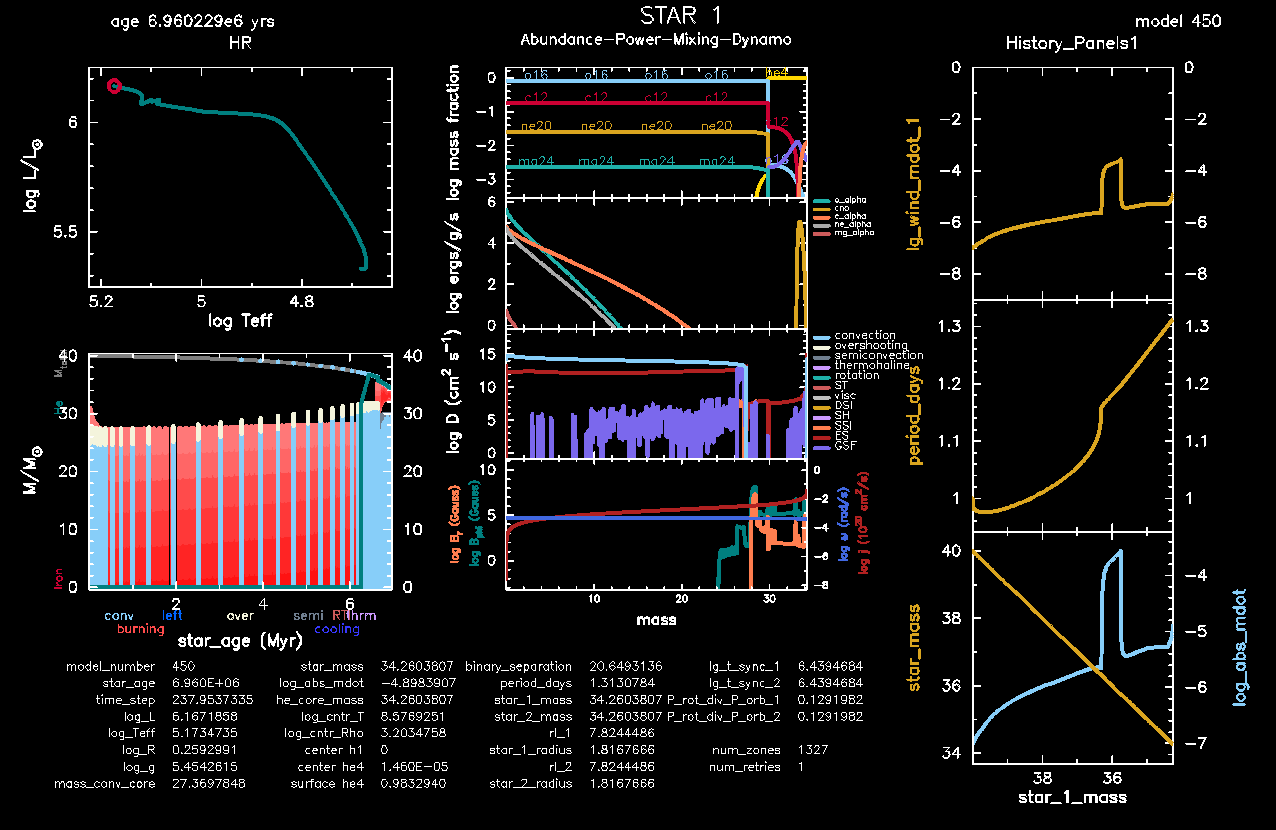
A star, in contrast, has very strong mass-loss, greater spin-down, and clearly shifts into a differentially-rotating structure, with flattening out and falling near the surface, as seen below.
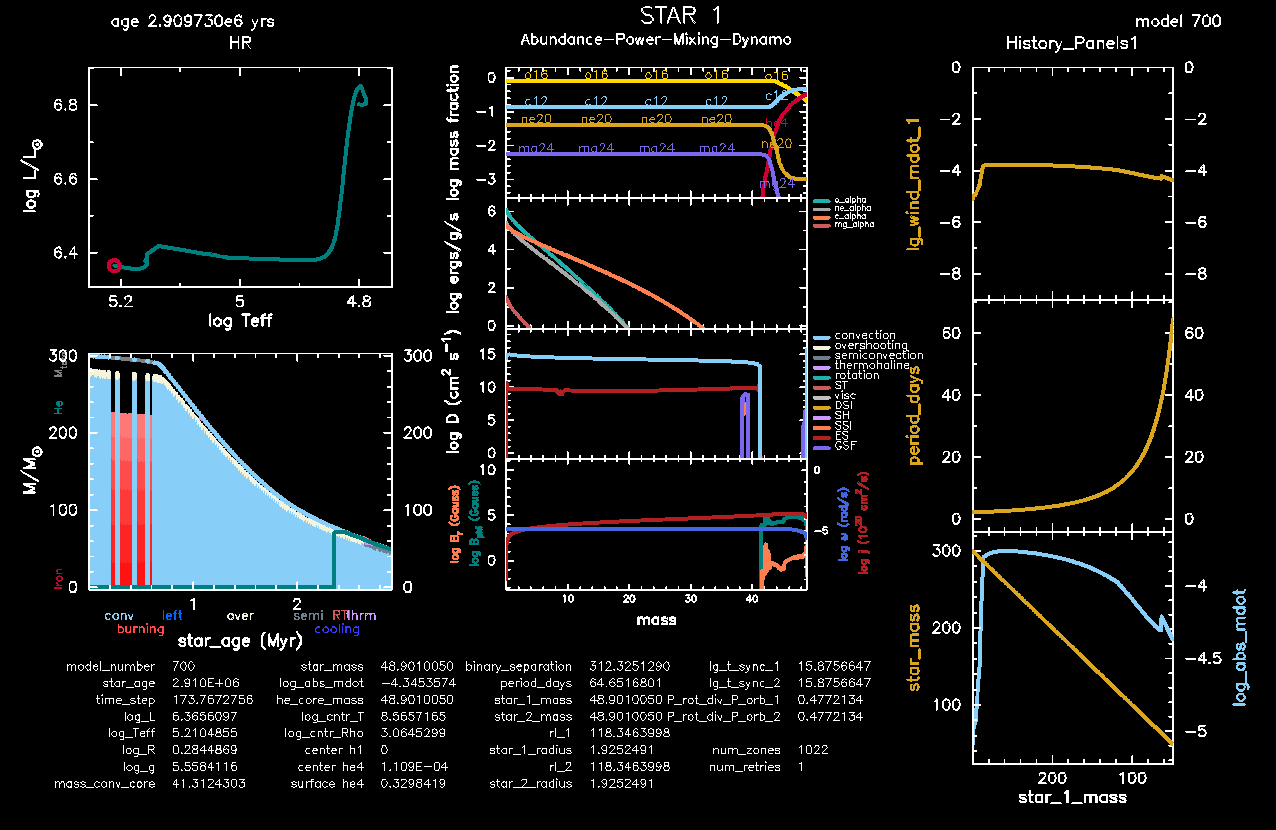
The development of differential rotation is closely linked to angular momentum (AM) transport inside the star, which will try to redistribute AM away from high- to low- regions. So far we have used the Tayler-Spruit dynamo, which for a wide range of masses is enough to keep the star rigidly rotating to the end of He burning. The Tayler-Spruit dynamo is the main mechanism through which the innermost region can be spun down (rather than the surface only), and thus is directly connected to the eventual BH spin.
./re and the initial controls
initial and non-initial pair, such as change_initial_model_twins_flag and change_model_twins_flag. In these cases, the former is applied only on a brand new run (./rn) while the latter gets reapplied in restarts as well (./re). Only set a pure change_*_flag to .true. if you are sure you want it to override potentially different settings on a restart!If you finish Move 3 ahead of time, you can also have a look at the bonus exercise at the end of the lab.
If you need to catch up, find a full solution of Move 3 here.
Move 4: open position into underarm twirl, or the He core spin

CHE stars keep spinning even after drifting apart into open position.
We will next use the mass and spin of our CHE stars at the end of He burning to estimate the produced BH masses and spins. The BH dimensionless spin parameter, (sometimes called ), is defined as
and takes on values between (non-spinning) and (maximally spinning).
We are going to implement a new history column through run_star_extras named chi_he_core that will track
for the He core. While our CHE stars are already almost one big He core (such that the core mass and spin are essentially the total mass and spin), explicitly looking for the He core boundary will allow the same column to be used for stars with a hydrogen envelope later.
To implement a new column in run_star_extras, we will rely on a few quantities that are internally computed in mesa and available through a star_info object, instantiated as s. Scalar quantities stored in s can be recovered as s% property_name, while arrays can be recovered as s% array_name(index or indices). The available properties are listed in $MESA_DIR/star_data/public.
Note
MESA arrays run from the surface to the center. The index of the innermost “shell” corresponds to the total number of zones into which the star is divided, which is stored as s% nz. Fortran arrays can be sliced as array(index1:index2).
For calculating physical quantities, MESA already includes a large collection of physical constants in CGS in the const_def library. This library is already imported by default in run_star_extras and its constants, which you can find in const/public/, can be used directly.
MESA already finds and stores information about the He core boundary for us, so to start we just want to note down how to get the numbers we need to compute .
Browse through
star_data/publicto find relevant parameters at the He core boundary. Keep an eye out for any quantities that are not stored in CGS; these cases are highlighted explicitly.Hint
Try runninggrep -rin he_coreinsidestar_data/public.Solution
We find in
star_data/public/star_data_step_work.incthe list of available quantities computed by MESA at the He core boundary,! abundance boundaries real(dp) :: he_core_mass ! baryonic (Msun) real(dp) :: he_core_radius ! Rsun real(dp) :: he_core_lgT real(dp) :: he_core_lgRho real(dp) :: he_core_L ! Lsun real(dp) :: he_core_v real(dp) :: he_core_omega ! (s^-1) real(dp) :: he_core_omega_div_omega_crit integer :: he_core_k ! boundary is in this cellWhile the mass is there, we are missing AM. We have, however, the index at the core boundary, meaning we could compute it if we had the AM profile.
Note also that
he_core_massis in Msun, not grams. We can convert it to the CGS by multiplying it byMsunlater.We will need to compute the He core total AM ourselves by integrating the specific AM from the center to the He core boundary,
Look for the necessary arrays (
j_rot(k), anddm(k)) again instar_data/public. How would you write out the slice of these arrays that captures the He core?Hint
Try runninggrep -rin "angular momentum"insidestar_data/public.Solution
The specific AM array is defined in
star_data/public/star_data_step_input.inc,! rotation real(dp), pointer, dimension(:) :: j_rot ! (nz) ! j_rot(k) is specific angular momentum at outer edge of cell k; = i_rot*omegaWhile the array — here, the mass per shell — is in
star_data/public/star_data_work_input.increal(dp), pointer :: dm(:) ! dm(k) is baryonic mass of cell k ! dm(k) = s% dq(k)*s% xmstarThis means you can call the am slice as:
s% j_rot(s% he_core_k : s% nz)and the corresponding mass slice as
s% dm(s% he_core_k : s% nz)Tell MESA to expect an extra history column in
src/run_star_extras.f90
Hint
how_many_extra_history_columnsSolution
Simply increase how_many_extra_history_columns to 2,
   integer function how_many_extra_history_columns(id)
      integer, intent(in) :: id
      integer :: ierr
      type (star_info), pointer :: s
      ierr = 0
      call star_ptr(id, s, ierr)
      if (ierr /= 0) return
      how_many_extra_history_columns = 2
end function how_many_extra_history_columns- Add the
chi_he_corecolumn by changing thedata_for_extra_history_columnssubroutine inrun_star_extras.f90.
Remember to look for constants inconst/publicif you need them.Hint 1: constants
You will useclightandstandard_cgravfor constants. Remember that the constants, specific AM and shell masses (dm) are already in CGS!Hint 2: integration
Since MESA discretizes stellar structure, your integral will be a sum over the product of thej_rotanddmarrays. Element-wise array products are implemented inmath_libwithdot_product, and array slices can be taken asarray(i1:i2).
Solution
In data_for_extra_history_columns, compute
and with that the dimensionless spin parameter of the core.
Then you can name that column and add the computed spin value. Your final implementation should look approximately like this.
   subroutine data_for_extra_history_columns(id, n, names, vals, ierr)
      integer, intent(in) :: id, n
      character (len=maxlen_history_column_name) :: names(n)
      real(dp) :: vals(n)
      integer, intent(out) :: ierr
      real(dp) :: dt, chi_he_core, J_he_core
      type (star_info), pointer :: s
      ierr = 0
      call star_ptr(id, s, ierr)
      if (ierr /= 0) return

      ! note: do NOT add the extras names to history_columns.list
      ! the history_columns.list is only for the built-in history column options.
      ! it must not include the new column names you are adding here.

      dt = dble(time1 - time0) / clock_rate / 60
      names(1) = 'runtime_minutes'
      vals(1) = dt

      ! NEW
      if (s% he_core_k == 0) then
         ! no He core yet
         chi_he_core = 0d0
      else
         J_he_core = dot_product(s% j_rot(s% he_core_k : s% nz),  s% dm(s% he_core_k : s% nz))
         ! Msun is solar mass in grams, used to convert he_core_mass
         chi_he_core = clight * J_he_core / (standard_cgrav * s% he_core_mass * s% he_core_mass * Msun * Msun)
      end if

      names(2) = 'chi_he_core'
      vals(2) = chi_he_core

   end subroutine data_for_extra_history_columns
Once you have included your new column, go ahead and recompile MESA by running ./mk in your work folder. Remember you have to do this every time you change any files inside src/. If you run into errors while compiling and are not sure what you did wrong, don’t hesitate to ask for help!
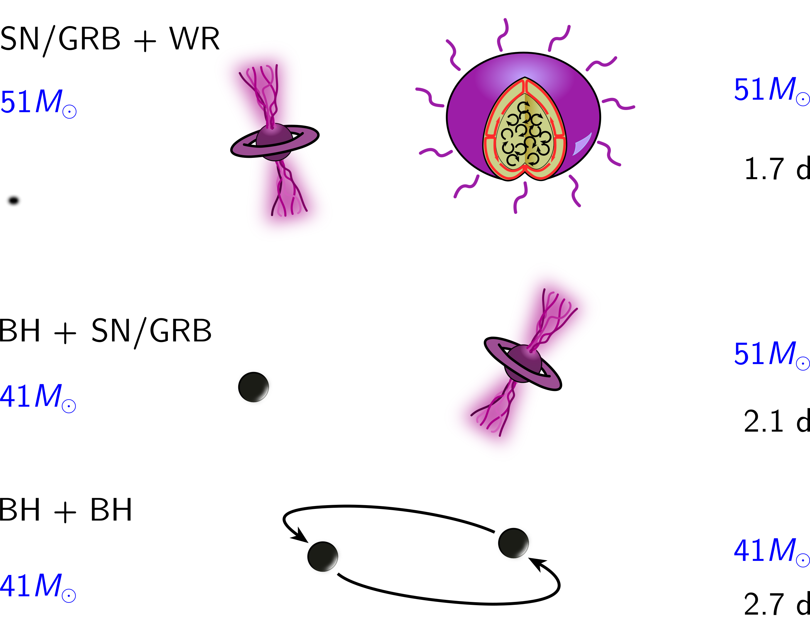
Schematic of the late stages of a CHE binary, at which point the stars are Wolf-Rayets (WRs), and result in a supernova (SN) and/or gamma-ray burst (GRB).
Add your newly created column to the text summary in pgplot by modifying the Luckily the last row on column 4 is free, so it is enough to add,&pgstar settings in inlist_star.Solution
Text_Summary1_name(8,4) = 'chi_he_core'
For seeing your new column in action, we would like to test the effect of different AM transport mechanisms on the final BH spins. For this, we will try either turning the TS dynamo off completely, or applying a flat intensity modifier; both can be achieved through the am_nu_ST_factor control in inlist_star.
Choose one of four AM transport alternatives to implement (or keep). Coordinate with your neighbors to pick different ones. The model tag will be used later.
| AM transport model | Model tag | Settings |
|---|---|---|
| No TS | nu0 | am_nu_ST_factor=0 |
| 0.001x TS | nu0001 | am_nu_ST_factor=0.001d0 |
| 1x TS | nu1 | am_nu_ST_factor=1d0 |
| 1000x TS | nu1000 | am_nu_ST_factor=1000d0 |
- Run your model!
Because we are changing fundamental physics, this time we will have to restart the entire run from ZAMS, which you can do by simply calling
./rn. Expect that the run will take at least 10 minutes, which you can use to read ahead on the final crowd-sourcing exercise, or discuss your results with your colleagues.
Warning
The entire run should still take 10 to 15 minutes, most of it spent in the MS. If you notice your run is past 10 minutes and your star still has not reached hydrogen depletion (check the center_h1), ask for someone to have a look. For the next step you can always use the final profile from Move 3, which corresponds to the 1x TS model.
Once your run is concluded, you might find that !? How do you interpret this?
Solution
 The reason we are able to find
is that we do not actually have a BH with
. Rather, we have a
He core, which is very far from the relativistic regime. What we are finding is more precisely put as: if all the mass and AM in this He core were to turn into a BH, it would have
. Since we expect this cannot happen in Nature, the conclusion is that not all the mass and AM can actually make it into the eventual BH. In Move 5 we deal with what could happen then.
The reason we are able to find
is that we do not actually have a BH with
. Rather, we have a
He core, which is very far from the relativistic regime. What we are finding is more precisely put as: if all the mass and AM in this He core were to turn into a BH, it would have
. Since we expect this cannot happen in Nature, the conclusion is that not all the mass and AM can actually make it into the eventual BH. In Move 5 we deal with what could happen then.Regardless of what you find, this is only a very rough approximation for what kind of BH will eventually be produced. We can do one better by accounting for the AM structure of the star in the last Move.
If you need to catch up, find a full solution of Move 4 here.
Move 5: now switch partners! or crowd-sourcing BH spins

Starting in 1920s Harlem, swing is a community dance, and so is science! There are too many reasonable physics assumptions and moves for any one person to try them all.
The innermost stable circular orbit (ISCO) is the smallest stable orbit around a BH, and sets the truncation radius of an accretion disk. Assuming the innermost form a seed BH at core-collapse, we can walk outward through the star and ask for each mass shell: is the specific AM of this shell greater than the corresponding , assuming an orbit around all the mass interior to this point?
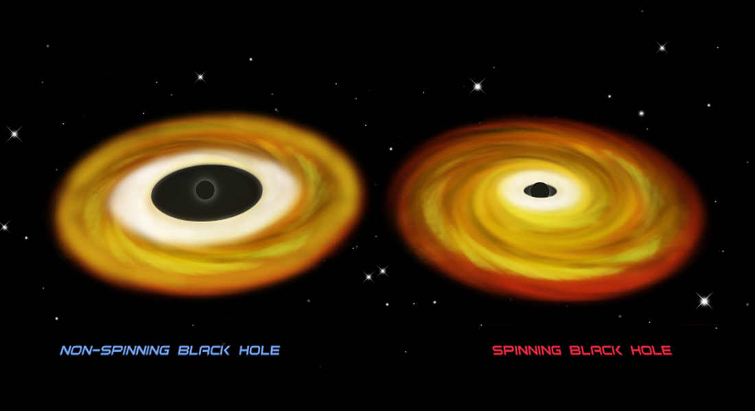
A BH's accretion disk is truncated sharply at ISCO in this representation. By definition, orbits below ISCO are unstable and matter falls in directly. Spinning (Kerr) BHs have smaller ISCO radii. Credit: NASA/CXC/M.Weiss
Anywhere where cannot be accreted onto the BH without losing AM first and is likely to settle into a disk before being accreted or ejected. While we cannot simulate a disk, we can estimate the prompt BH mass and spin, which is the seed mass + the sum of mass shells fulfilling . To do this we start at the layer enclosing , and find the first layer above it where . Everything between the two can be added to the seed BH. This breaks any sort of simple mapping between the stellar spin and the BH spin.
As we will see it is not trivial to form a highly-spinning BH from a highly-spinning star!
A Colab notebook has been prepared in order to compute that mass and show you the of all your final models in this Drive folder. Please rename your last profile.data file according to the instructions, then upload it to that folder.
Important
In order to create labels, the notebook reads your physical settings from the file name. The file you upload should be named NAME_mX_AMy.data, where you should replace NAME with your name, X with your mass (integer) and y with your AM transport model tag from the table above. For example, if I ran the
star with the 1x TS AM transport model, I would upload my last profile with the name lucas_m70_AMnu1.data.
After uploading your profile, you can try running the notebook online by following the instructions within. It should automatically pick up your file and that of any colleagues (if not, check the naming), add it to plot, and compute the prompt mass and spin. Can you explain the emerging patterns over mass and AM transport?
Why ?
The motivation comes from solving Einstein’s equations for the general case of a BH with mass , AM and electric charge (this is called a Kerr-Newman solution). Demanding that the solution include an event horizon around the singularity yields the condition
The hypothesis that Nature does not produce so-called naked singularities is called the Cosmic Censorship hypothesis and is tacitly assumed everywhere when is imposed. This is a hard constraint on the three numbers that fully define a BH (that the three numbers , , suffice is called the No Hair Theorem). Further defining,
also encodes the assumption that the BH is electrically neutral, which follows reasonably from stellar evolution.
Conclusions
By the end of this lab, we have encountered first-hand the most dramatic difference between CHE and non-CHE stars, and how post-MS evolution can decouple the surface and core rotation rates. We have also learned how to compute the BH spin corresponding to a He core, and how that assumption does not trivially hold.
Bonus exercises
If you have extra time, here are some extra things you can try at the end of a few of the Moves.
In Move 2
You can try to map out exactly the range that leads to CHE for your mass! Try going both up and down from the tabulated period. If your run is stopped before reaching the end of the MS, note the termination message. What was the reason? This should tell you whether you need to move the period up or down to achieve a CHE star, and what physically limits the period range.
Hint
There are only a few termination messages you should be getting during this run. If you seeTerminate due to primary not evolving homogeneously, that means your star is not spinning rapidly enough and needs to be in a closer orbit. If you seetermination code: Terminate because of overflowing initial model(or L2 overflow), it means your stars are so close they would have undergone an episode of likely unstable mass transfer and merged; in this case, you need a wider orbit.By trying a different mass yourself, or comparing with colleagues, determine how the period range behaves with mass. Does it close anywhere? The constraints on mass and period together make up the “CHE window”.
Solution
For our setup, there is effectively no room left for CHE by , and the range is already much narrower for stars than for . The CHE window is bounded below in mass, and both above (by slow rotation) and below (by L2 overflow) in period.There is a particular behavior in the HR diagram that emerges with increasing mass: at some point, the mass-loss rate suddenly starts to increase, and the uptick in mass-loss causes your star to dip down in luminosity sharply. This is related to a particular ingredient in our custom wind scheme turning on. Can you figure out which, and why it is characteristic of higher masses?
3Solution
This behavior is a direct consequence of the inclusion of MS optically-thick winds in our setup from theeval_Vink2011_wind, which are normally characteristic of very massive stars ( ), but can get triggered at lower masses for CHE. The trigger comes from reaching a switch value for the Eddington factor. Because luminosity scales steeply with mass and , the switch is more easily reachable the more massive the star is. CHE makes the switch even easier because the helium opacity to electron scattering is lower, making a CHE star more luminous for a fixed mass.
In Move 3
Looking at the post-MS HR and Kippenhahn diagrams: would it be accurate to say that your star never expands at all? Why? Compare your results to neighbors running different masses, both during and after the MS. Do their tracks look very different from yours?Hint HR diagram
Hint Kippenhahn diagram