Lab 3: Stable relationships
This lab renders better with the light theme!
Introduction
In this last lab3 we will pick up on the system you evolved in lab1 and follow its further evolution into a double black hole binary. Remember that at the end of your lab1 you had two systems:
- One system underwent mass transfer during the Main Sequence (Case A mass transfer), with final properties listed in the below Table 1.
- The other underwent mass transfer after the Main Sequence (Case B mass transfer), with final properties as in Table 2.
| Primary (Stripped star) | Secondary (Accretor) | |
|---|---|---|
| Mass | 16.8 M☉ | 39.6 M☉ |
| Orbital Period | 4.5 days | |
| Mass ratio | 0.42 | |
| Final model | final1_caseA.mod | final2_caseA.mod |
| Primary (Stripped star) | Secondary (Accretor) | |
|---|---|---|
| Mass | 17.14 M☉ | 40.8 M☉ |
| Orbital Period | 32.2 days | |
| Mass ratio | 0.42 | |
| Final model | final1_caseB.mod | final2_caseB.mod |
Both these systems have a rapidly rotating (spun-up) secondary that has accreted a lot of mass from the primary; it is, therefore, “rejuvenated” (fresh fuel has prolonged its Main Sequence lifetime), and is happily burning hydrogen (H) in its core. The primary, on the other hand, has already depleted helium (He) in its core and has been “stripped” off its H-rich envelope.
Important
Notice that the Case A system has a much lower orbital period than the Case B. These different post-mass transfer properties determine a different further evolutionary history! In this lab3, we will understand how both types of binaries need to evolve in order to form gravitational wave sources such as merging binary black holes. They will evolve with a further stage of mass transfer, which may be
- STABLE: relatively long-lived (on the thermal or even nuclear timescale of the donor) and self regulated, with a quiet detachment afterwards.
- UNSTABLE: or “Common envelope”, a fast (~dynamical timescale) stage in which the envelope of the donor engulfs the binary.
- PART C: Common envelope evolution ⏰~20-30 minutes⏰
PART A: Stable mass transfer
Let’s copy the standard work directory from $MESA_DIR to your preferred local folder:
cp -r $MESA_DIR/binary/work stable_MT
cd stable_MT
Inspect your inlist_project and pay attention to the following two controls:
evolve_both_starsWhen false, MESA will model just one star, and keep the other as a point mass. This is convenient for binaries with compact objects, like black holes (BH). You can find more info here:$MESA_DIR/binary/defaults/binary_job.defaultslimit_retention_by_mdot_eddWhen true, the accretion rate of material onto the point-mass companion will be capped to a physical limit, called “Eddington limit”. This is because the infall of hot stellar material onto a compact object creates radiation pressure that may halt the accretion process. In this case, the excess transferred mass is ejected from the binary with the specific angular momentum of the point mass. You can find more info here:$MESA_DIR/binary/defaults/binary_controls.defaults
Our simulation is already set up to model one of the components as a point mass with Eddington limited accretion. Ideal starting point for us to model a binary with a BH.
SETUP: Eddington-limited accretion
Now we will perform some adjustments to the template. A significant number of these are meant to make the simulation faster in order to be efficiently computed in the duration of this lab.
Modify history_columns.list
Grab the history_columns.list file from $MESA_DIR/star/defaults and copy it into your work folder:
cp -r $MESA_DIR/star/defaults/history_columns.list .We will add an option to this file to visualize the quantities in the Kippenhahn diagram in the pgstar window. Search through this file for the string mixing_regions. Add below:
mixing_regions 10Modify binary_controls in inlist_project
By default MESA also includes the effect of magnetic braking for angular momentum loss. This implementation is meant for late type stars (see the Monday lab1, where you’ve seen the Kraft break 😌) and should be removed when working with massive binaries. Additionally, by default MESA reduces the growth of the BH mass to account for the rest-mass energy radiated away during accretion, determined by a radiative efficiency parameter. For simplicity, in this lab we will switch this control off. For these purposes, you can include:
! be 100% sure magnetic braking is always off
do_jdot_mb = .false.
! don't reduce the BH accretion efficiency
use_radiation_corrected_transfer_rate = .false.
To run the simulation faster we will relax multiple timestepping controls of the binary module by including:
! relax timestep controls
fm = 0.1d0
fa = 0.02d0
fa_hard = 0.04d0
fr = 0.5d0
fj = 0.01d0
fj_hard = 0.02d0
The exact purpose of each of these controls can be checked in the defaults file $MESA_DIR/binary/defaults/binary_controls.defaults, but in general fm, fa, fr and fj control the fractional change of envelope mass, binary separation, Roche lobe overfilling factor, and orbital angular momentum.
Finally, let’s add some options for the output of our simulation:
! output preferences
photo_interval = 50
history_interval = 1
Modify controls in inlist1
We will add a lot of options here that involve the individual stripped star model. Most of them are purely to make the run faster; we add also a prescription for the convective overshooting and a terminating condition at core-Helium depletion. Going through everything is beyond the scope of this lab (we are focusing on binaries here 🙃 and you have seen many of these already in the previous days), but feel free to dig into them later if you have time! Remember that the exact purpose of each of these controls can be checked in the defaults file $MESA_DIR/star/defaults/controls.defaults.
Modified controls for inlist1
&controls

   extra_terminal_output_file = 'log1'
   log_directory = 'LOGS1'

   ! we use step overshooting
   overshoot_scheme(1) = 'step'
   overshoot_zone_type(1) = 'burn_H'
   overshoot_zone_loc(1) = 'core'
   overshoot_bdy_loc(1) = 'top'
   overshoot_f(1) = 0.345
   overshoot_f0(1) = 0.01

   ! a bit of exponential overshooting for convective core during He burn
   overshoot_scheme(2) = 'exponential'
   overshoot_zone_type(2) = 'burn_He'
   overshoot_zone_loc(2) = 'core'
   overshoot_bdy_loc(2) = 'top'
   overshoot_f(2) = 0.01
   overshoot_f0(2) = 0.005

   use_ledoux_criterion = .true.
   alpha_semiconvection = 1d0

   ! stop when the center mass fraction of h1 drops below this limit
   ! relax default dHe/He, otherwise growing convective regions can cause things to go at a snail pace
   dX_limit_species(1) = 'he4'
   dX_div_X_limit(1) = 5d0
   dX_div_X_limit_min_X(1) = 1d-1
   ! we're not looking for much precision at the very late stages
   dX_nuc_drop_limit = 5d-2
   ! stop when the center mass fraction of he4 drops below this limit
   xa_central_lower_limit_species(1) = 'he4'
   xa_central_lower_limit(1) = 1d-2

   ! reduce resolution and solver tolerance to make runs faster
   mesh_delta_coeff = 3d0
   time_delta_coeff = 3d0
   varcontrol_target = 1d-2
   use_gold2_tolerances = .false.
   use_gold_tolerances = .true.

   ! Use scaled corrections to aid the solver
   scale_max_correction = 0.03d0
   ignore_min_corr_coeff_for_scale_max_correction = .true.
   ignore_species_in_max_correction = .true.
   scale_max_correction_for_negative_surf_lum = .true.

   use_superad_reduction = .true.
   eps_mdot_leak_frac_factor = 0d0

   ! output options
   profile_interval = 500
   history_interval = 1
   terminal_interval = 1
   write_header_frequency = 10
   max_num_profile_models = 10000

/ ! end of controls namelist
Modify pgstar in inlist1
Playing with pgstar can be very entertaining, but for this lab we will use a pre-made window. You can copy all this content and replace the default entirely:
Nice pgstar window
&pgstar

   pgstar_interval = 1

   pgstar_age_disp = 2.5
   pgstar_model_disp = 2.5

   !### scale for axis labels
   pgstar_xaxis_label_scale = 1.3
   pgstar_left_yaxis_label_scale = 1.3
   pgstar_right_yaxis_label_scale = 1.3

   Grid2_win_flag = .true.

   Grid2_win_width = 15
   Grid2_win_aspect_ratio = 0.65 ! aspect_ratio = height/width

   Grid2_plot_name(4) = 'Mixing'

   Grid2_num_cols = 7 ! divide plotting region into this many equal width cols
   Grid2_num_rows = 8 ! divide plotting region into this many equal height rows
   Grid2_num_plots = 6 ! <= 10

   Grid2_plot_name(1) = 'TRho_Profile'
   Grid2_plot_row(1) = 1 ! number from 1 at top
   Grid2_plot_rowspan(1) = 3 ! plot spans this number of rows
   Grid2_plot_col(1) =  1 ! number from 1 at left
   Grid2_plot_colspan(1) = 2 ! plot spans this number of columns
   Grid2_plot_pad_left(1) = -0.05 ! fraction of full window width for padding on left
   Grid2_plot_pad_right(1) = 0.01 ! fraction of full window width for padding on right
   Grid2_plot_pad_top(1) = 0.00 ! fraction of full window height for padding at top
   Grid2_plot_pad_bot(1) = 0.05 ! fraction of full window height for padding at bottom
   Grid2_txt_scale_factor(1) = 0.65 ! multiply txt_scale for subplot by this


   Grid2_plot_name(5) = 'Kipp'
   Grid2_plot_row(5) = 4 ! number from 1 at top
   Grid2_plot_rowspan(5) = 3 ! plot spans this number of rows
   Grid2_plot_col(5) =  1 ! number from 1 at left
   Grid2_plot_colspan(5) = 2 ! plot spans this number of columns
   Grid2_plot_pad_left(5) = -0.05 ! fraction of full window width for padding on left
   Grid2_plot_pad_right(5) = 0.01 ! fraction of full window width for padding on right
   Grid2_plot_pad_top(5) = 0.03 ! fraction of full window height for padding at top
   Grid2_plot_pad_bot(5) = 0.0 ! fraction of full window height for padding at bottom
   Grid2_txt_scale_factor(5) = 0.65 ! multiply txt_scale for subplot by this
   Kipp_title = ''
   Kipp_show_mass_boundaries = .true.

   Grid2_plot_name(6) = 'HR'
   HR_title = ''
   Grid2_plot_row(6) = 7 ! number from 1 at top
   Grid2_plot_rowspan(6) = 2 ! plot spans this number of rows
   Grid2_plot_col(6) =  6 ! number from 1 at left
   Grid2_plot_colspan(6) = 2 ! plot spans this number of columns

   Grid2_plot_pad_left(6) = 0.05 ! fraction of full window width for padding on left
   Grid2_plot_pad_right(6) = -0.01 ! fraction of full window width for padding on right
   Grid2_plot_pad_top(6) = 0.0 ! fraction of full window height for padding at top
   Grid2_plot_pad_bot(6) = 0.0 ! fraction of full window height for padding at bottom
   Grid2_txt_scale_factor(6) = 0.65 ! multiply txt_scale for subplot by this

   History_Panels1_title = ''
   History_Panels1_num_panels = 3

   History_Panels1_xaxis_name='model_number'
   History_Panels1_max_width = -1 ! only used if > 0.  causes xmin to move with xmax.

   History_Panels1_yaxis_name(1) = 'period_days'
   History_Panels1_other_yaxis_name(1) = ''
   History_Panels1_yaxis_log(1) = .true.
   History_Panels1_yaxis_reversed(1) = .false.
   History_Panels1_ymin(1) = -101d0 ! only used if /= -101d0
   History_Panels1_ymax(1) = -101d0 ! only used if /= -101d0
   !History_Panels1_dymin(1) = 0.1

   History_Panels1_yaxis_name(2) = 'lg_mtransfer_rate' !
   History_Panels1_yaxis_reversed(2) = .false.
   History_Panels1_ymin(2) = -8d0 ! only used if /= -101d0
   History_Panels1_ymax(2) = -1d0 ! only used if /= -101d0
   History_Panels1_dymin(2) = 1

   ! ADD THE L2 MASS OUTFLOW RATE TO THE HISTORY PANEL
   History_Panels1_other_yaxis_name(2) = ''
   History_Panels1_other_yaxis_reversed(2) = .false.
   History_Panels1_other_ymin(2) = -8d0 ! only used if /= -101d0
   History_Panels1_other_ymax(2) = -1d0 ! only used if /= -101d0
   History_Panels1_other_dymin(2) = 1

   History_Panels1_yaxis_name(3) = 'rl_relative_overflow_1'
   History_Panels1_other_yaxis_name(3) = ''
   History_Panels1_yaxis_reversed(3) = .false.

   Grid2_plot_name(2) = 'Text_Summary1'
   Grid2_plot_row(2) = 7 ! number from 1 at top
   Grid2_plot_rowspan(2) = 2 ! plot spans this number of rows
   Grid2_plot_col(2) = 1 ! number from 1 at left
   Grid2_plot_colspan(2) = 4 ! plot spans this number of columns
   Grid2_plot_pad_left(2) = -0.08 ! fraction of full window width for padding on left
   Grid2_plot_pad_right(2) = -0.10 ! fraction of full window width for padding on right
   Grid2_plot_pad_top(2) = 0.08 ! fraction of full window height for padding at top
   Grid2_plot_pad_bot(2) = -0.04 ! fraction of full window height for padding at bottom
   Grid2_txt_scale_factor(2) = 0.19 ! multiply txt_scale for subplot by this
   Text_Summary1_name(7,1) = 'period_days'
   Text_Summary1_name(8,1) = 'star_2_mass'
   Text_Summary1_name(7,4) = ''

   ! ADD THE TDELAY TO THE TEXT SUMMARY
   Text_Summary1_name(8,4) = ''

   Grid2_plot_name(3) = 'Profile_Panels3'
   Profile_Panels3_title = 'Abundance-Power-Mixing'
   Profile_Panels3_num_panels = 3
   Profile_Panels3_yaxis_name(1) = 'Abundance'
   Profile_Panels3_yaxis_name(2) = 'Power'
   Profile_Panels3_yaxis_name(3) = 'Mixing'

   Profile_Panels3_xaxis_name = 'mass'
   Profile_Panels3_xaxis_reversed = .false.

   Grid2_plot_row(3) = 1 ! number from 1 at top
   Grid2_plot_rowspan(3) = 6 ! plot spans this number of rows
   Grid2_plot_col(3) = 3 ! plot spans this number of columns
   Grid2_plot_colspan(3) = 3 ! plot spans this number of columns

   Grid2_plot_pad_left(3) = 0.09 ! fraction of full window width for padding on left
   Grid2_plot_pad_right(3) = 0.07 ! fraction of full window width for padding on right
   Grid2_plot_pad_top(3) = 0.0 ! fraction of full window height for padding at top
   Grid2_plot_pad_bot(3) = 0.0 ! fraction of full window height for padding at bottom
   Grid2_txt_scale_factor(3) = 0.65 ! multiply txt_scale for subplot by this

   Grid2_plot_name(4) = 'History_Panels1'
   Grid2_plot_row(4) = 1 ! number from 1 at top
   Grid2_plot_rowspan(4) = 6 ! plot spans this number of rows
   Grid2_plot_col(4) =  6 ! number from 1 at left
   Grid2_plot_colspan(4) = 2 ! plot spans this number of columns
   Grid2_plot_pad_left(4) = 0.05 ! fraction of full window width for padding on left
   Grid2_plot_pad_right(4) = 0.03 ! fraction of full window width for padding on right
   Grid2_plot_pad_top(4) = 0.0 ! fraction of full window height for padding at top
   Grid2_plot_pad_bot(4) = 0.07 ! fraction of full window height for padding at bottom
   Grid2_txt_scale_factor(4) = 0.65 ! multiply txt_scale for subplot by this

   Grid2_file_flag = .true.
   Grid2_file_dir = 'png1'
   Grid2_file_prefix = 'grid_'
   Grid2_file_interval = 1 ! 1 ! output when mod(model_number,Grid2_file_interval)==0
   Grid2_file_width = -1 ! negative means use same value as for window
   Grid2_file_aspect_ratio = -1 ! negative means use same value as for window

/ ! end of pgstar namelist
Also add pause_before_terminate = .true. to &star_job just below pgstar_flag = .true. if you’d like to take a moment to admire your final pgstar window after every run.
Get final1_caseA.mod and final2_caseA.mod
Grab the final models final1_caseA.mod and final2_caseA.mod from Table 1 and copy them into your work folder.
The stripped star becomes a BH companion
After He depletion in its core, the stripped star has a very short remaining lifetime: for a star of total mass ~ 20 (and He-core mass of ~ 10 ), you can expect it to live only another ~ 300 years! For simplicity, we will just assume that the properties at core He depletion can be representative of those at the end of the star’s life. Additionally, we will assume that all the mass contained in the primary directly collapses to form a BH.
inlist_projectFind the mass of the stripped star at core He depletion from your lab1 and, assuming it directly collapses into a BH, set its mass in inlist_project. Set also the period of your binary to be the one you found at the end of lab1.
💡 How do I find the BH mass?
Your inlist_project already has evolve_both_stars = .false., so one of the two stars will be treated as a point mass –> BH!
To find the mass of this BH, you can open the final1_caseA.mod and look at the header.
💡 m1 or m2?
Remember which one was stripped in lab1 (the primary, final1_caseA.mod), and which one was accreted (the secondary, final2_caseA.mod). The stripped star will become the BH (m2), and the accretor will become your new primary (m1).
Solution
   m1 = 39.6d0 ! primary mass in Msun
   m2 = 16.8d0 ! BH mass in Msun
   initial_period_in_days = 4.5d0 ! final period from lab1
Now you have set up the properties of your binary system. We are only missing one piece: we need to load the model of the accretor from lab1 as our new primary star.
inlist1Load the right model from your lab1 in your inlist1.
💡 Which command is it?
Checking inside $MESA_DIR/star/defaults/star_job.defaults. You can search for the string load…
Solution
Inside your inlist1:
&star_job
   ...
   load_saved_model = .true.
   load_model_filename = 'final2_caseA.mod'
   ...
/ ! end of star_job namelist
Note
Did you need to set both masses in inlist_project? Nope! Since you loaded a pre-computed model for your new primary (the accretor of lab1), its mass and properties will be read directly from the model final2_caseA.mod. However, you still need to set the BH mass!
Computing the time delay
Compact binaries composed of neutron stars and BHs gradually lose orbital energy through the emission of gravitational waves. As a consequence, the orbit shrinks over time until the two compact objects eventually merge.
The gravitational-wave time delay (or simply delay time) is the time required for this inspiral and merger to occur if gravitational-wave emission were the only process acting on the binary orbit. Delay times are particularly important in astrophysics because they determine when mergers happen relative to the formation of the stars, and therefore affect the populations of gravitational-wave sources observed by detectors such as LIGO, Virgo and KAGRA1.
For a circular orbit, the merger timescale derived by Peters (1964)2 is
where:
- is the orbital separation at the BH + BH stage;
- and are the masses of the two BHs,
- is the gravitational constant,
- is the speed of light.
Notice the strong dependence : even modestly wider binaries can take dramatically longer to merge. The dependence on the masses is a bit weaker, but the rule of thumb is that more massive systems will merge faster.
In practice, delay times are often expressed in Gigayears (Gyr), where years, because this makes it easy to compare them to the age of the Universe Gyr). This comparison tells us whether a compact binary has enough time to merge within cosmic history: binaries with Gyr may merge and be observable today as gravitational-wave sources, while systems with longer delay times are effectively undetectable (technically, they have “not yet happened” anywhere in the Universe 🤓).
Note
Remember that so far, you have initialized a system with a star + BH, since you have collapsed all the mass of the stripped star of lab1 into a point mass m2, and initialized your m1 to be the accretor of lab1. After evolving your system further, your m1 will reach Helium depletion in its core, and at the point it will very close to become the second BH of your system: that’s how you will achieve a BH + BH binary! From that point onwards, the
calculation will make sense, as the interaction between the two BHs is expected to be only via gravity.
Important
In principle, BHs can accrete mass (and in fact, that is when they become X-Ray active 🌝), and this option in your inlist_project
limit_retention_by_mdot_edd = .true.will make such that the accretion rate onto the BH is Eddington-limited (we talked about it in here). This is a standard assumption when treating BH accretors, which is observationally motivated by beautiful systems like the galactic microquasar SS433, where powerful relativistic jets are thought to drive material away from the central binary. However, keep in mind that this is not exact science and there are other possible ways to treat (and limit) accretion onto BHs: we will explore one further down in the lab.
run_binary_extras.f90Let’s compute the
in Gigayears (Eq. (1)) as an extra binary history column tdelay(Gyr) in run_binary_extras.f90, and print its value on the pgstar window, in the Text Summary part. Here’s a reminder of the formula you need to use:
💡 Mind the units...
In stellar astrophysics and in MESA we like to use the centimeter-gram-second units, therefore we saved our own useful constants to convert between energy units, or from seconds to years, and such.
Those constants are readily accessible in run_star_extras.f90, if you know what their name is 🙃
You may want to use:
clight, the speed of light in cm/ssecyer, the conversion between years and secondsstandard_cgrav, the gravitational constant in c.g.s.
Loaded via: use const_def
See also: $MESA_DIR/const/public/const_def.f90
💡 Fighting with the binary pointer b% ?
Don’t be scared, the binary_info structure and its type b work very similarly to the star_info and its type s! Try to find the quantities of interest inside $MESA_DIR/binary/public/binary_data.inc, and refer to them with the pointers b% m(1), b% m(2), ecc. Pay attention to the units!
Solution for run_binary_extras.f90
subroutine data_for_extra_binary_history_columns(binary_id, n, names, vals, ierr)
  type(binary_info), pointer :: b
  integer, intent(in) :: binary_id
  integer, intent(in) :: n
  character(len=maxlen_binary_history_column_name) :: names(n)
  real(dp) :: vals(n)
  integer, intent(out) :: ierr
  ierr = 0
  call binary_ptr(binary_id, b, ierr)
  if (ierr /= 0) then
      write (*, *) 'failed in binary_ptr'
      return
  end if

  names(1) = 'tdelay(Gyr)'
  vals(1) = (5d0/256d0) * (clight**5 * b%separation**4) / &
        (standard_cgrav**3 * b%m(1) * b%m(2) * (b%m(1) + b%m(2)))

  ! convert from seconds -> years -> Gyr
  vals(1) = vals(1) / secyer / 1d9

end subroutine data_for_extra_binary_history_columns
integer function how_many_extra_binary_history_columns(binary_id)
use binary_def, only: binary_info
integer, intent(in) :: binary_id
how_many_extra_binary_history_columns = 1
end function how_many_extra_binary_history_columns💡 Too many pgstar things to look at?
Search for the string “TDELAY” in inlist1 😏
Solution for pgstar
! ADD THE TDELAY TO THE TEXT SUMMARY
Text_Summary1_name(8,4) = 'tdelay(Gyr)'
RUN 1
You have come a long way, congrats! We are finally ready to start our first run.
Warning
Never forget to do ./clean and ./mk after modifying the run_binary_extras.f90 file.
Your pgstar window should look like something like this (this is the very last png, from the last model of your run, model 749):
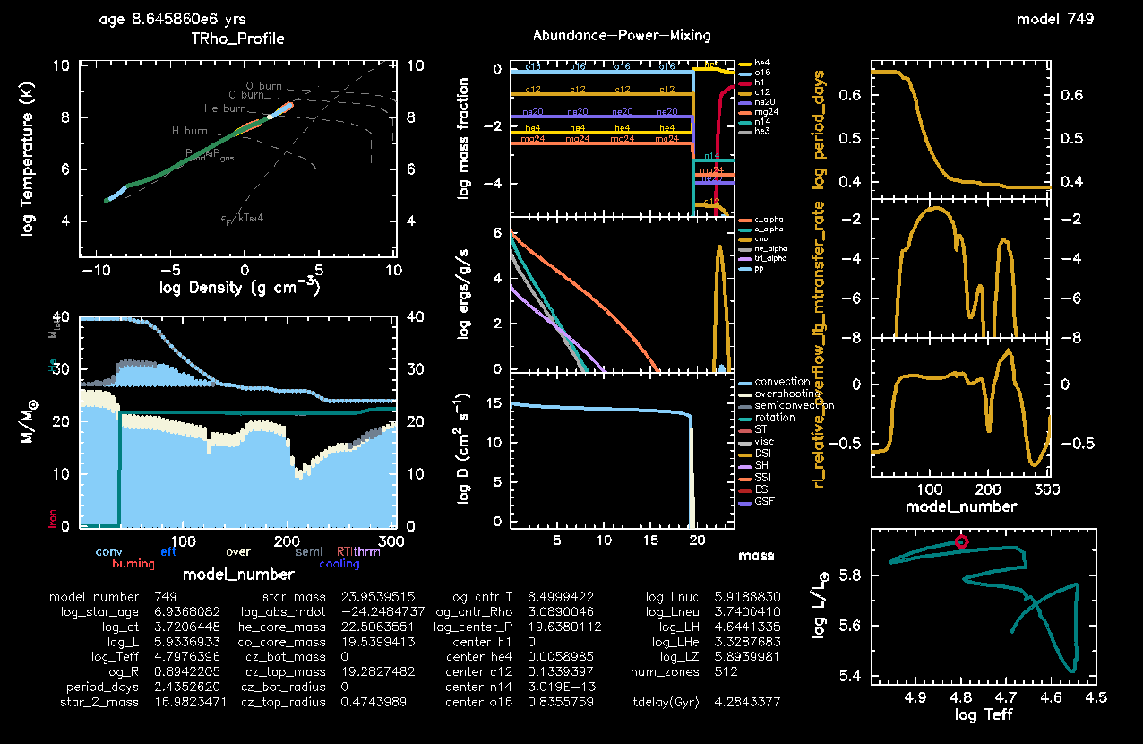
Figure 1. Stable mass transfer, Case A evolution for a star + BH binary (click to zoom in!).
- Make sure that the Kippenhahn diagram shows nice convective zones (filled in light blue) and the Helium core (the solid green line). If it is the case, you did well in putting
mixing_regions 10inhistory_columns.list(as indicated in this section) ☺️ Otherwise, no problem. Do it now, as we will look into the Kippenhahn diagram for a later run. You can also download the correct filehere. - Check that the info about the
tdelay(Gyr)column is appearing in the Text Summary, as you can see in here. If not, you may have done something wrong with the implementation… You can try again, but if you’re short on time, just look at Figure 1 (click to zoom in!) to answer to the Discuss the run questions here below.
Discuss the run: Case A mass transfer!
Here are some discussion points for you to understand what happened physically to your star + BH system; you will only need to look at Figure 1 (click to zoom in!). Try to think about it and answer together with your table.
Which type of mass transfer do you observe in this star + BH run?
Solution
The mass transfer starts during the Main Sequence → Case A! You can see it from the shape of the Hertzsprung-Russel diagram (ask your TA if you don’t know!).How much mass did the donor star lose?
Solution
The donor star started from a mass of (see Table 1), and is now . You can read this value in the Text Summary (star_mass), or look at the Kippenhahn diagram. So it lost , which corresponds to 40% of its initial mass!Is the donor star stripped to its core?
Solution
Almost! Look at the Text Summary (he_core_mass) and / or the Kippenhahn diagram. The Helium core is , and the donor is stripped to a total mass of . The Helium core amounts to 93.9% of the star, while the Hydrogen-rich envelope amounts to , only 6.1%.How much mass did the BH accrete? Do you understand why?
Solution
The BH accretor started from a mass of (see Table 1), and is now (seestar_2_massvalue). Therefore it only accreted , so it increased its mass by only 1.1%. The Eddington-limited accretion made such that the mass transfer becomes almost completely non-conservative (i.e., all the material is expelled from the binary).How did the orbit evolve during mass transfer? And what is the final period?
Solution
The system started with a period of days, and has followed a sort of parabola-shaped path (see thelog_period_daysplot) that has led to shrinkage. At the end of the mass transfer episode, the orbit is days wide. This amounts to almost 50% overall shrinkage!Assume that the donor star will collapse into a BH of mass equal to its mass at Helium depletion (end of the run). Will the system merge within the age of the Universe?
Solution
You have calculated thetdelay(Gyr)yourself 🌝 You see it is equal to 4.28 Gyr, less than the age of the Universe ( ). Yes, we have chirping binary black holes!How is the final mass ratio of your BH + BH binary?
Solution
The donor will collapse into a BH of mass , and the companion BH has a mass of . The mass ratio is then ! This number is right about what more detailed population synthesis studies expect for stable mass transfer to produce 😌
PART B: Stable mass transfer 2.0
SETUP: Orbital tightening from L2 mass loss
So far, we have considered an Eddington-limited mass-transfer scenario, in which matter that cannot be accreted by the black hole is expelled from the vicinity of the accretor itself. This is the so-called isotropic re-emission mode. In this picture, the expelled material removes the specific angular momentum of the accretor from the binary system.
However, this is not the only possible way for matter to leave the binary. 3D hydrodynamical simulations 3 show that when the mass-transfer rate becomes sufficiently high (roughly ), some of the transferred material can instead be lifted all the way to the second Lagrangian point, . This is the Lagrangian point located on the far side of the less massive object in the binary (see Figure 2).
Because the point is located farther away from the center of mass than the accretor itself, material escaping through carries away much more angular momentum than in the isotropic re-emission case.
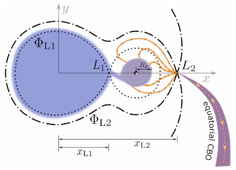 Figure 2. Schematics3 of
outflow in a binary, where the
s indicate different levels of gravitational equipotential;
is the first Lagrangian point (through which material can flow).
Figure 2. Schematics3 of
outflow in a binary, where the
s indicate different levels of gravitational equipotential;
is the first Lagrangian point (through which material can flow).
In practice, this introduces an additional contribution to the orbital angular momentum evolution of the binary system, which for simplicity we will write as
where these is the time derivative of the angular momentum component (and “ml” = mass loss). The angular momentum loss associated with matter expelled through the point can be written as
while the standard isotropic re-emission contribution is
Here:
- is the mass transfer rate
- is the orbital separation,
- is the orbital period,
- is the position of the point in units of the orbital separation,
- is the fraction of transferred mass expelled through isotropic re-emission,
- is the fraction expelled through the outflow channel.
These efficiency factors determine how conservative the mass transfer is:
- → all transferred material is expelled from the system → THIS WILL BE OUR CASE IN THIS PART B!
- → fully conservative mass transfer (everything is retained in the system).
- → this plays the same role as that you saw in lab1 (where is for conservative mass transfer, and is fully non-conservative), but this time it is modified to our purpose of having only two types of mass leakage: the isotropic re-emission mode, and overflow.
Curiosity: observational motivation of outflows 🌀
Important
In the context of gravitational wave sources, mass outflow is expected to efficiently tighten star + BH binaries that are residing in quite wide orbits, so that after the detachment, the binary will be already close enough to start chirping at the formation of the second BH! In this part of the lab3, we will demonstrate that, in presence of mass outflow, a wide binary, like the Case B system you produced in lab1, can form a gravitational wave source after stable mass transfer.
You can start from the same setup as you developed so far (also downloadable here):
cp -r stable_MT stable_MT_L2Remind yourself of the properties of your Case B system in Table 2, and download the final1_caseB.mod and final2_caseB.mod. You see that the masses are mostly the same, but you will have to change the period, and load the right model 😎Solution for
inlist_project&binary_controls
...
m1 = 40.8d0 ! donor mass in Msun
m2 = 17.14d0 ! companion mass in Msun
initial_period_in_days = 32.2d0
...
/ ! end of binary_controls namelistSolution for
inlist1&star_job
...
load_saved_model = .true.
load_model_filename = 'final2_caseB.mod'
...
/ ! end of star_job namelist
Additionally, we still have the Eddington-limited mass accretion rate switched on, like we wanted to in our first part of the lab. But now we want to introduce our own prescription for how the mass outflows from the system, introducing
outflow! Therefore, we set this to .false. now in inlist_project
limit_retention_by_mdot_edd = .false.run_binary_extras.f90Let’s make such that our binary will lose 35% of transferred material through the second Lagrangian point
(
), and the rest 65% will be lost from the vicinity of the accretor (
). You will need to introduce two personalized routines: my_jdot_ml and my_adjust_mdots, and an x_ctrl(1) in inlist1. This is a difficult task, so don’t be scared and read all the hints!
🎁 Let's find L2 in run_binary_extras.f90
This is a gift for you (or simply, something you can find in literature 4 and you don’t need to know how to code on the spot 🤙🏻). Copy this entirely at the end of your run_binary_extras.f90.
Routine to copy into run_binary_extras.f90
! ROCHE POTENTIAL FIRST DERIVATIVE
! To find the Lagrangian points numerically, by bisection
real(dp) function dPhidx(b,x) result(derivative)
real(dp), intent(in) :: x
real(dp) :: q, x_cm
type(binary_info), pointer :: b
! include 'formats.inc'

q = b% m(b% d_i)/b% m(b% a_i)
x_cm = 1/(1+q)
derivative = 1/(x*abs(x)) +1/(q*(x-1)*abs(x-1)) -(x-x_cm)*(q+1)/q

end function dPhidx


! FUNCTION TO FIND THE COORDINATE OF L2 IN UNITS OF SEPARATION
real(dp) function find_L2(b) result(L2)
real(dp) :: limit, tolerance, x, upper_bound, lower_bound, dPhi_new,q
type(binary_info), pointer :: b
! include 'formats.inc'

q = b% m(b% d_i)/b% m(b% a_i)

if (q < 1) then
  upper_bound = 0d0
  lower_bound = -1d0
  limit = abs(upper_bound-lower_bound)/abs(lower_bound)
end if

if (q .GE. 1) then
  upper_bound = 2d0
  lower_bound = 1d0
  limit = abs(upper_bound-lower_bound)/abs(upper_bound)
end if

x = 0d0

tolerance = 0.000001d0

do while (limit > tolerance)
  x = (lower_bound+upper_bound)/2
  dPhi_new = dPhidx(b,x)
  if (dPhi_new > 0) then
      lower_bound = x
  else if (dPhi_new < 0) then
      upper_bound = x
  else
      exit
  end if

  if (q < 1) then
      limit = abs(upper_bound-lower_bound)/abs(lower_bound)
  end if

  if (q .GE. 1) then
      limit = abs(upper_bound-lower_bound)/abs(upper_bound)
  end if

end do
L2 = (upper_bound + lower_bound)/2
end function find_L2
💡 35% of mass lost via L2?
We can make use of an x_ctrl(1) to set the fraction of mass that is lost from the system removing the specific angular momentum of the
point!
Solution for inlist1
&controls
  ...
  x_ctrl(1) = 0.35d0
  ...
/ ! end of controls namelist
💡 How to lose the remaining 65%?
To set the fraction
of mass that is leaving the system with the specific angular momentum of the accretor (isotropic re-emission mode), there is actually a default control that you can look up in $MESA_DIR/binary/defaults/binary_controls.defaults. You can look for the string beta 🙃
Solution for inlist_project
&binary_controls
  ...
  ! transfer efficiency controls
   limit_retention_by_mdot_edd = .false.
   mass_transfer_beta = 0.65d0
  ...
/ ! end of controls namelist
💡 Is all mass lost in the way that I want?
In $MESA_DIR/binary/defaults/binary_controls.defaults, give a look at the meaning and the default values of all these controls: mass_transfer_alpha, mass_transfer_delta, mass_transfer_gamma. What are their default values?
Additionally, remember that you have set this in inlist_project
limit_retention_by_mdot_edd = .false.Solution: yes 😛
As you saw in lab1, these fractions
,
and
describe other possible leakages of mass, which we are not interested in. Luckily, they are all set to zero by default! So the only one that we have set is
, as wanted. The remaining 0.35 mass outflow will be calculated by us with our own personalized fraction
(or x_ctrl(1)).
Additionally, the Eddington limit is switched off, so that we are in full control of where 35%+65%=100% of the mass goes!
💡 Activating new run_binary_extras.f90 hooks
We are going to create our own personalized run_binary_extras.f90 routines to compute the orbital evolution due to mass losses from the system (jdot_ml equation) and the changes in mass due to accretion / leakages (mdots equation). We need to instruct inlist_project to use the new routines! Try to find the right controls in $MESA_DIR/binary/defaults/binary_controls.defaults. You can look for the string use_other_.
Solution for inlist_project
&binary_controls
  ...
  ! ADD personalized run_binary_extras.f90 routine
  use_other_jdot_ml = .true.
  use_other_adjust_mdots = .true.
  ...
/ ! end of binary_controls namelist
💡 Set the function pointers in run_binary_extras.f90
As usual when we activate personalized hooks in run_binary_extras.f90, we also need to instruct extras_binary_controls to point to those new routines, that we will call my_adjust_mdots and my_jdot_ml.
Solution for extras_binary_controls
subroutine extras_binary_controls(binary_id, ierr)
  ...
  ...
  ! EXTRA SHRINKAGE FOR L2 MASS OUTFLOW!
  ! Default routine: $MESA_DIR/binary/private/binary_jdot.f90
  ! But the empty hook from where you usually start is:
  ! $MESA_DIR/binary/other/mod_other_binary_jdot.f90
  b% other_jdot_ml => my_jdot_ml

  ! Default routine: $MESA_DIR/binary/private/binary_mdot.f90
  ! But the empty hook from where you usually start is:
  ! $MESA_DIR/binary/other/mod_other_adjust_mdots.f90
  b% other_adjust_mdots => my_adjust_mdots
  ...
  ...
end subroutine extras_binary_controls
Nice, you’ve completed the easy part! The further two steps (in red) are difficult. you will need to create the run_binary_extras.f90 routines for my_jdot_ml and my_adjust_mdots from scratch. If you are tired and / or short on time, no problem! Please read the hints and try think about it by yourself for at least a few minutes. But don’t feel bad to look at the solutions 😊
Note
To compute the orbital evolution due to mass losses from the system (jdot_ml equation) and the changes in mass due to accretion / leakages (mdots equation), MESA uses two default routines:
default_jdot_ml, to be found in$MESA_DIR/binary/private/binary_jdot.f90. If you want to create your own personalized version of it, the empty hook from where you usually start is:$MESA_DIR/binary/other/mod_other_binary_jdot.f90adjust_mdots, to be found in$MESA_DIR/binary/private/binary_mdot.f90. If you want to create your own personalized version of it, the empty hook from where you usually start is:$MESA_DIR/binary/other/mod_other_adjust_mdots.f90
💡 Creating my_adjust_mdots → DIFFICULT!
Start by copying this guided skeleton entirely inside your run_binary_extras.f90. This is just a commented version of the classic empty routine null_other_adjust_mdots from $MESA_DIR/binary/other_mod_other_adjust_mdots.f90!
Guided skeleton of my_adjust_mdots
subroutine my_adjust_mdots(binary_id, ierr)
  use binary_def, only : binary_info, binary_ptr
  use const_def, only: dp
  integer, intent(in) :: binary_id
  integer, intent(out) :: ierr
  type (binary_info), pointer :: b
  real(dp) :: fixed_xfer_fraction
  ierr = 0
  call binary_ptr(binary_id, b, ierr)
  if (ierr /= 0) then
  write(*,*) 'failed in binary_ptr'
  return
  end if

  ! THIS IS WHERE YOU CAN IMPOSE THE MASS TRANSFER FRACTION
  ! In your lab1, this looked like:
  ! epsilon = 1 - alpha - beta - delta - gamma.
  ! In this lab3, we want to only model beta (isotropic re-emission)
  ! and upsilon (L2 outflow), while all the rest is already set to zero
  ! in the defaults.
  b% fixed_xfer_fraction = 0d0    !!!modify this


  ! EDDINGTON ACCRETION RATE
  ! Usually, one should also eval mdot_edd here by calling the default
  ! functions using the ones provided through binary_lib.
  ! But in our lab3, we want to ignore Eddington limits anyway...
  b% mdot_edd = 0d0
  b% mdot_edd_eta = 0d0


  ! WIND MASS TRANSFER EFFICIENCY
  ! Usually, one should also eval the wind mass transfer efficiency
  ! here by calling the default functions provided through binary_lib.
  ! But we want to ignore wind mass transfer for simplicity...
  b% mdot_wind_transfer(:) = 0d0
  b% wind_xfer_fraction(:) = 0d0


  ! MASS CHANGES IN THE TWO STARS DUE TO MASS TRANSFER
  ! Set mdot for the donor
  b% s_donor% mstar_dot = 0d0     !!!modify this
  ! Set mdot for the accretor
  ! point_mass_i is 0 if both stars are evolved, is 1 if there is a BH!
  if (b% point_mass_i == 0) then
      b% component_mdot(b% a_i) = 0d0
  else
      b% component_mdot(b% a_i) = 0d0   !!!modify this
  end if
  ! Accretion luminosity is useful only if you have a compact
  ! accretor and want to use it to compute the Eddington limit,
  ! but you can set it to zero if you want to ignore that...
  b% accretion_luminosity = 0d0


  ! mdot_system_transfer is mass lost from the vicinity of each star;
  ! such mass will be removing the angular momentum of the respective star.
  ! We want to model this for the accretor (you can access it via
  ! b% mdot_system_transfer(b% a_i)), this is the
  ! isotropic re-emission mode! But we want to ignore it for the donor.
  b% mdot_system_transfer(:) = 0d0    !!!modify this

  ! mdot_system_cct is mass lost from a circumbinary coplanar toroid.
  ! we are not interested in modeling this one :)
  b% mdot_system_cct = 0d0

  end subroutine my_adjust_mdots
Read all the comments and try to fill in where you see !!! modify this. Keep in mind the following:
You have set your with the control
mass_transfer_beta, and your withx_ctrl(1). You can access quantities related to your donor from thebinary_infostructure asb% s_donor!The donor should have an
mdotthat corresponds to the mass transfer rate (which is defined negative, since it loses mass!)The accretor should have an
mdotthat corresponds to a fraction of the mass transfer rate (and which sign?)
Solution for my_adjust_mdots
subroutine my_adjust_mdots(binary_id, ierr)
    use binary_def, only : binary_info, binary_ptr
    use const_def, only: dp
    integer, intent(in) :: binary_id
    integer, intent(out) :: ierr
    type (binary_info), pointer :: b
    real(dp) :: fixed_xfer_fraction
    ierr = 0
    call binary_ptr(binary_id, b, ierr)
    if (ierr /= 0) then
    write(*,*) 'failed in binary_ptr'
    return
    end if

    ! THIS IS WHERE YOU CAN IMPOSE THE MASS TRANSFER FRACTION
    ! In your lab1, this looked like:
    ! epsilon = 1 - alpha - beta - delta - gamma.
    ! In this lab3, we want to only model beta (isotropic re-emission)
    ! and upsilon (L2 outflow), while all the rest is already set to zero
    ! in the defaults.
    b% fixed_xfer_fraction = 1 - b% mass_transfer_beta - b% s_donor% x_ctrl(1)    !!!modify this


    ! EDDINGTON ACCRETION RATE
    ! Usually, one should also eval mdot_edd here by calling the default
    ! functions using the ones provided through binary_lib.
    ! But in our lab3, we want to ignore Eddington limits anyway...
    b% mdot_edd = 0d0
    b% mdot_edd_eta = 0d0


    ! WIND MASS TRANSFER EFFICIENCY
    ! Usually, one should also eval the wind mass transfer efficiency
    ! here by calling the default functions provided through binary_lib.
    ! But we want to ignore wind mass transfer for simplicity...
    b% mdot_wind_transfer(:) = 0d0
    b% wind_xfer_fraction(:) = 0d0


    ! MASS CHANGES IN THE TWO STARS DUE TO MASS TRANSFER
    ! Set mdot for the donor
    b% s_donor% mstar_dot = b% mtransfer_rate     !!!modify this
    ! Set mdot for the accretor
    ! point_mass_i is 0 if both stars are evolved, is 1 if there is a BH!
    if (b% point_mass_i == 0) then
        b% component_mdot(b% a_i) = 0d0
    else
        b% component_mdot(b% a_i) = -b% mtransfer_rate* b% fixed_xfer_fraction   !!!modify this
    end if
    ! Accretion luminosity is useful only if you have a compact
    ! accretor and want to use it to compute the Eddington limit,
    ! but you can set it to zero if you want to ignore that...
    b% accretion_luminosity = 0d0


    ! mdot_system_transfer is mass lost from the vicinity of each star;
    ! such mass will be removing the angular momentum of the respective star.
    ! We want to model this for the accretor (you can access it via
    ! b% mdot_system_transfer(b% a_i)), this is the
    ! isotropic re-emission mode! But we want to ignore it for the donor.
    b% mdot_system_transfer(b% d_i) = 0d0
    b% mdot_system_transfer(b% a_i) = b% mtransfer_rate * b% mass_transfer_beta    !!!modify this

    ! mdot_system_cct is mass lost from a circumbinary coplanar toroid.
    ! we are not interestered in modeling this one :)
    b% mdot_system_cct = 0d0

end subroutine my_adjust_mdots
💡 Creating my_jdot_ml → DIFFICULT!
This is the part in which you will use Eq. (2) and Eq. (3).
Start by copying this guided skeleton entirely inside your run_binary_extras.f90. This is just a commented version of the classic empty routine null_other_jdot_ml from $MESA_DIR/binary/other/mod_other_binary_jdot.f90!
Guided skeleton of my_jdot_ml
subroutine my_jdot_ml(binary_id, ierr)
  use binary_def, only : binary_info, binary_ptr
  integer, intent(in) :: binary_id
  integer, intent(out) :: ierr
  type (binary_info), pointer :: b
  ierr = 0
  call binary_ptr(binary_id, b, ierr)
  if (ierr /= 0) then
  write(*,*) 'failed in binary_ptr'
  return
  end if

  ! THIS IS WHERE YOU CAN IMPOSE THE ANGULAR MOMENTUM LOSS RATE
  ! ASSOCIATED WITH MASS LOSS
  ! Remember that you have two types of mass loss:
  ! the isotropic re-emission mode (beta) and the L2 outflow (upsilon).
  ! The first one is already implemented in MESA,
  ! we just need to find how to write it.
  ! Look at the default routine that MESA uses in
  ! $MESA_DIR/binary/private/binary_jdot.f90, and copy the relevant piece.
  ! You can also check the formula that we wrote on the website for Jdot_isotropic, it should correspond :)
  b% jdot_ml = 0      !!!leave this like that and modify below
  b% jdot_ml = b% jdot_ml +  ...  !!!modify this

  ! Now add the L2 outflow contribution, which is not included in the default MESA jdot routine, so you will have to write it from scratch using the formula on the website!
  ! Watch out: in the formula, you will need to find the coordinate of L2 in units of separation, which is not a built-in MESA quantity, but you can calculate it using the function find_L2 that we provided as a gift!
  b% jdot_ml = b% jdot_ml +  ...     !!!modify this

end subroutine my_jdot_ml
Read all the comments and try to fill in where you see !!! modify this.
Solution for my_jdot_ml
subroutine my_jdot_ml(binary_id, ierr)
    use binary_def, only : binary_info, binary_ptr
    integer, intent(in) :: binary_id
    integer, intent(out) :: ierr
    type (binary_info), pointer :: b
    real(dp) :: x_L2
    ierr = 0
    call binary_ptr(binary_id, b, ierr)
    if (ierr /= 0) then
    write(*,*) 'failed in binary_ptr'
    return
    end if

    ! THIS IS WHERE YOU CAN IMPOSE THE ANGULAR MOMENTUM LOSS RATE
    ! ASSOCIATED WITH MASS LOSS
    ! Remember that you have two types of mass loss:
    ! the isotropic re-emission mode (beta) and the L2 outflow (upsilon).
    ! The first one is already implemented in MESA,
    ! we just need to find how to write it.
    ! Look at the default routine that MESA uses in
    ! $MESA_DIR/binary/private/binary_jdot.f90, and copy the relevant piece.
    ! You can also check the formula that we wrote on the website for Jdot_isotropic, it should correspond :)
    b% jdot_ml = 0d0
    b% jdot_ml = b% jdot_ml + b% mdot_system_transfer(b% a_i)*&
    pow2(b% m(b% d_i)/(b% m(b% a_i)+b% m(b% d_i))*b% separation)*2*pi/b% period *&
    sqrt(1 - pow2(b% eccentricity))

    ! Now add the L2 outflow contribution, which is not included in the default MESA jdot routine, so you will have to write it from scratch using the formula on the website!
    ! Calculate the coordinate of L2 in units of separation
    x_L2 = abs(find_L2(b))
    ! Add the contribution to jdot from mass lost from L2
    b% jdot_ml = b% jdot_ml + (b% mtransfer_rate * b% s_donor% x_ctrl(1))*&
    ((b% m(b% a_i)/(b% m(b% a_i)+b% m(b% d_i))-x_L2)*b% separation)**2*2*pi/b% period

end subroutine my_jdot_ml
💡 Showing the L2 rate on pgstar
Final touch: visualization of the (log of) the mass loss from
in our pgstar window. We will need to modify the data_for_extra_binary_history_columns and how_many_extra_binary_history_columns in run_binary_extras.f90 as usual.
Don’t forget that b% mtransfer_rate is negative, and is in cgs units. Invoke the constants Msun and secyer!
Solution for run_binary_extras.f90
   subroutine data_for_extra_binary_history_columns(binary_id, n, names, vals, ierr)
      type(binary_info), pointer :: b
      integer, intent(in) :: binary_id
      integer, intent(in) :: n
      character(len=maxlen_binary_history_column_name) :: names(n)
      real(dp) :: vals(n)
      integer, intent(out) :: ierr
      ierr = 0
      call binary_ptr(binary_id, b, ierr)
      if (ierr /= 0) then
         write (*, *) 'failed in binary_ptr'
         return
      end if

      names(1) = 'tdelay(Gyr)'
      vals(1) = (5d0/256d0) * (clight**5 * b%separation**4) / &
      (standard_cgrav**3 * b%m(1) * b%m(2) * (b%m(1) + b%m(2)))

      ! convert from seconds -> years -> Gyr
      vals(1) = vals(1) / secyer / 1d9

      ! L2 mass outflow rate in Msun/yr
      names(2) = "lg_mdot_L2"
      ! Let's take the log of the absolute value
      vals(2) = log10(abs((b% mtransfer_rate * b% s_donor% x_ctrl(1) )/Msun*secyer))

   end subroutine data_for_extra_binary_history_columns
integer function how_many_extra_binary_history_columns(binary_id)
use binary_def, only: binary_info
integer, intent(in) :: binary_id
how_many_extra_binary_history_columns = 2
end function how_many_extra_binary_history_columnsSolution for inlist1
! ADD THE L2 MASS OUTFLOW RATE TO THE HISTORY PANEL
History_Panels1_other_yaxis_name(2) = 'lg_mdot_L2'
RUN 2
Warning
Don’t forget to do ./clean and ./mk after modifying the run_binary_extras.f90 file.
Your pgstar window should look like something like this (this is the very last png, from the last model of your run, model 712):
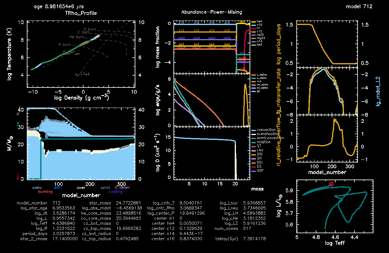
Figure 3. Stable mass transfer, Case B evolution for a star + BH binary (click to zoom in!).
- Make sure the mass loss rate from is appearing in your mass transfer rate plot. If it looks like Figure 3, you must have done everything right 🍻🍻
Discuss the run: Case B mass transfer!
Here are some discussion points for you to understand what happened physically to your star + BH system; you will only need to look at Figure 3 (click to zoom in!). Try to think about it and answer together with your table.
- Which type of mass transfer do you observe in this star + BH run?
Solution
The mass transfer starts after the Main Sequence → Case B! You can see it from the shape of the Hertzsprung-Russel diagram (ask your TA if you don’t know!). - How much mass did the donor star lose? How is it compared to the previous run that was assuming Eddington-limited accretion?
Solution
The donor star started from a mass of (see Table 1), and is now . You can read this value in the Text Summary (star_mass), or look at the Kippenhahn diagram. So it lost , which corresponds to 40% of its initial mass! More or less, like in the Case A system. - How much mass did the BH accrete? Any difference with the previous run?
Solution
The BH accretor started from a mass of (see Table 1), and is now… (seestar_2_massvalue)! It accreted absolutely nothing, as we wanted. Our setup is constructed such that , i.e. 100% of the mass that the donor transfers is expelled from the binary. - How much did the orbit shrink? Compare with the previous run.
Solution
The system started with a period of days. At the end of the mass transfer episode, the orbit is days wide. This amounts to 91% overall shrinkage! Quite wild, and for sure wilder than the Eddington-limited case. - Will the system merge within the age of the Universe?
Solution
We have in this case a time delay of Gyr. So yes, another chirping binary! - How is the final mass ratio of your BH + BH binary? Any difference with the previous run?
Solution
The donor will collapse into a BH of mass , and the companion BH has a mass of . The mass ratio is then ! Not much difference with the previous run, and still consistent with population synthesis studies of stable mass transfer 😌
PART C: Common envelope evolution
Common envelope (CE) evolution is a phase during which the envelope of the donor star engulfs the whole binary. The embedded system experiences strong drag forces while orbiting inside the envelope, causing the orbit to shrink and orbital energy to be transferred to the gas. Friction, shocks, and recombination energy are thought to help unbind part of the envelope, often leaving behind circumstellar material around the system. Observationally, CE events are frequently associated with luminous red novae (see V1309 Sco, the “Rosetta stone” of this class of transients 💥).
CE occurs when mass transfer becomes unstable. This can happen in binaries with very extreme mass ratios (i.e. the donor is much more massive than the accretor), or when the donor star is highly evolved and possesses a deep convective envelope. In these situations, mass transfer may initially proceed stably, but the donor envelope may not be able to shrink fast enough to remain inside its Roche lobe. The resulting runaway increase in mass-transfer rate creates a positive feedback loop: mass loss shrinks the Roche lobe and simultaneously drives further expansion of the donor envelope. There is currently no consensus on the condition for when this process becomes irreversible (i.e., the actual CE onset), but a rule of thumb is to compare the mass-transfer rate to the Kelvin–Helmholtz timescale of the donor and define the onset of CE when
The final outcome of CE evolution is highly uncertain because the process is intrinsically three-dimensional and hydrodynamical (thus computationally expensive to simulate). In some cases the binary merges completely if the inspiral is too strong; in others, the envelope is successfully ejected and the binary survives with a much tighter orbit. In literature, the final orbital separation post-CE, , is commonly computed using the energy formalism5. In this framework, the binding energy of the donor envelope is assumed to be balanced by a fraction of the released orbital energy:
Solving for the post-CE separation gives
which is directly translatable into the post-CE period via the III Kepler’s law:
is the donor mass at CE onset, and is the mass of the donor envelope, such that one can assume , i.e. the remaining Helium core of the donor star,
and are the accretor masses at onset and post-CE, usually assumed to be equal: ,
is the orbital separation at CE onset,
is the orbital separation post-CE,
is the gravitational constant,
is the CE efficiency parameter, usually assumed to be ,
is the binding energy of the donor envelope. This can be estimated by integrating the gravitational and internal energy of the envelope layers:
and is the mass enclosed within a shell, is the radius of the shell, is the specific internal energy, is the correction due to molecular hydrogen dissociation energy, is the mass of the shell.
Important
In the context of gravitational wave sources, CE has been classically invoked as a way to form double BHs binaries, due to its efficient tightening of the orbit of star + BH systems prior to the evolution into BH + BH binaries. Pretty much as the stable mass transfer channels that we have seen above 😁 The aim of this exercise is to explore how CE evolution can form gravitational wave sources and compare its outcome to the stable mass transfer channel.
You can start from the same setup as you developed for the Case A mass transfer (also downloadable here):
cp -r stable_MT CERemind yourself of the properties of your Case A system in Table 1. In particular, look at the mass ratio:
. This is a very mild mass ratio, and in fact the mass transfer between star + BH was stable! Let’s change the BH mass to
: this gives us a very extreme mass ratio (
) that will favor CE evolution instead 😎Solution for
inlist_project&binary_controls
...
m1 = 39.6d0 ! donor mass in Msun
m2 = 5d0 ! companion mass in Msun
initial_period_in_days = 4.5d0
...
/ ! end of binary_controls namelist
Caution
In principle, if you ran your setup as is, it will work: the primary will evolve on its Main Sequence, initiate a Case A mass transfer episode, and reach very high mass transfer rates. MESA will start complaining with smaller and smaller timesteps, several retries, convergence issues. This regime is not only numerically challenging and expensive for the solver, but also quite meaningless, as CE is inherently a 3D-hydro process on the dynamical timescale and out of hydrostatic equilibrium!
Note
- MESA actually has a suite of routines for modeling the CE stage in 1D in the most physically-motivated possible way (mostly following the formalism from Marchant et al. (2021)4)! We will not make use of these, but if you are curious, you can give a look at last year’s Summer School binary day. We will instead stop our simulation at CE onset, and use the energy formalism to predict the post-CE properties of our binary.
- When you want to pass information between
run_star_extras.f90andrun_binary_extras.f90(for example, if you calculate something indata_for_extra_history_columnsand you want to use that quantity indata_for_extra_binary_history_columns), you can use thes% xtraarray! - If you don’t know how quantities are called, you can check
$MESA_DIR/star_data/public/star_data_step_work.incfor thes%structure, and$MESA_DIR/binary/public/binary_data.incfor theb%structure.
run_star_extras.f90Calculate an extra history column Ebind(erg) for the binding energy
of the hydrogen envelope of our star, in
(Eq. (7)). Then save its value into s% xtra. Here’s a reminder of the formula you need:
💡 Why is run_star_extras.f90 empty...?
Your run_star_extras.f90 looks kinda empty because it is running the standard routines in standard_run_star_extras.inc. We need to copy those routines in here and modify them. Do you remember where they are? You can always do a
`grep -nri standard_run_star_extras.inc $MESA_DIR/star`in your terminal and try to find the file yourself.
Solution
$MESA_DIR/star/job/standard_run_star_extras.inc in place of the line include 'standard_run_star_extras.inc'.💡 Remember how to loop?
You can loop over the star’s shells with a fortran loop from k=1 (surface) to k=s% nz (center). Watch out: in Eq. (7) you have an integral from the (He-rich) core of the star to the surface, so you’ll want your loop to go through only hydrogen-rich shells, to compute the Ebind of the envelope.
You can check whether the shells are hydrogen-rich with something like s% X(k) > 0.1d0, where s% X(k) is the hydrogen mass fraction at the mass shell k.
Skeleton of your loop
do k=1, s% nz
  if (s% X(k) > 0.1d0) then
      Ebind = ...
  else
      exit
  end if
end do
🎁 Gift: Hydrogen dissociation energy!
This is another gift for you (for the sake of time, but it is still an interesting exercise to get to know several MESA constants in $MESA_DIR/const/public/const_def.f90). This is how you can code the molecular hydrogen dissociation energy
in the calculation of Ebind(erg):
avo*4.52d0/2d0*ev2erg*s% X(k)Curious to understand why?
The hydrogen dissociation energy contribution enters the integrand of Eq. (7) as
Here
is the dissociation energy of molecular hydrogen,
(avo) is Avogadro’s number, ev2erg converts eV to erg, and
is the hydrogen mass fraction in each zone. The factor
accounts for the two hydrogen atoms per
molecule, giving the energy per gram of stellar material.
💡 Mind the units...
You want Eq. (7) to give you a quantity in
, the cgs unit for energy. So be sure to check all the units in $MESA_DIR/star_data/public/star_data_step_work.inc.
Full solution for Ebind(erg)
subroutine data_for_extra_history_columns(id, n, names, vals, ierr)
  integer, intent(in) :: id, n
  character (len=maxlen_history_column_name) :: names(n)
  real(dp) :: vals(n)
  real(dp) :: Ebind
  integer :: k
  integer, intent(out) :: ierr
  type (star_info), pointer :: s
  ierr = 0
  call star_ptr(id, s, ierr)
  if (ierr /= 0) return

  ! note: do NOT add the extras names to history_columns.list
  ! the history_columns.list is only for the built-in history column options.
  ! it must not include the new column names you are adding here.

  names(1)="Ebind(erg)"
  Ebind = 0d0
  do k=1, s% nz
    if (s% X(k) > 0.1d0) then
        Ebind = Ebind + s% dm(k)*(-standard_cgrav*s% m(k)/s% r(k)+s% energy(k)-avo*4.52d0/2d0*ev2erg*s% X(k))
    else
        exit
    end if
  end do
  vals(1) = Ebind
  s% xtra(1) = Ebind

end subroutine data_for_extra_history_columns
integer function how_many_extra_history_columns(id)
integer, intent(in) :: id
integer :: ierr
type (star_info), pointer :: s
ierr = 0
call star_ptr(id, s, ierr)
if (ierr /= 0) return
how_many_extra_history_columns = 1
end function how_many_extra_history_columnsrun_binary_extras.f90Let’s implement a stopping condition at the onset of the common envelope episode, i.e. when the mass transfer rate exceeds
(Eq. (4)), and let’s show the Kelvin-Helmholtz mass loss rate on the pgstar window together with lg_mtransfer_rate. Here’s a reminder of the Equation you need:
💡 MESA already computes kh_timescale 🤓
Surprise, you don’t need to compute
for Eq. (4), because there is an associated quantity to be found in $MESA_DIR/star_data/public/star_data_step_work.inc.
Solution
s% kh_timescale, and it’s in years.💡 Where do I put the stopping condition?
For a single star simulation, you would put it into the extras_finish_step routine… For a binary, it is very similar 🧠
Full stopping condition
integer function extras_binary_finish_step(binary_id)
  type(binary_info), pointer :: b
  type (star_info), pointer :: s
  integer, intent(in) :: binary_id
  integer :: ierr
  call binary_ptr(binary_id, b, ierr)
  if (ierr /= 0) then  ! failure in  binary_ptr
      return
  end if
  extras_binary_finish_step = keep_going

  if (abs(b% mtransfer_rate)*secyer/Msun > 10d0*b% s_donor% m(1) /Msun / b% s_donor% kh_timescale) then
      extras_binary_finish_step = terminate
      write(*,*) "Terminate due to mdot>10*M_kh: CE onset!"
  end if

  end function extras_binary_finish_step
💡 Visualizing on pgstar
We want to visualize the Kelvin-Helmholtz mass loss rate together with lg_mtransfer_rate, therefore we need to save the logarithm of
as an extra history column, called something like log10(Mdot_KH).
Additionally, we want to modify the pgstar namelist in inlist1 in a clever spot. I would put it where you put the
rate early on: search for the string “L2”
Solution for data_for_extra_binary_history_columns
Notice that we had already the calculation of tdelay(Gyr) from the first run. So you will have to also increase by 1 the count of how_many_extra_binary_history_columns.
subroutine data_for_extra_binary_history_columns(binary_id, n, names, vals, ierr)
  type(binary_info), pointer :: b
  integer, intent(in) :: binary_id
  integer, intent(in) :: n
  character(len=maxlen_binary_history_column_name) :: names(n)
  real(dp) :: vals(n)
  real(dp) :: a_postCE, P_postCE
  integer, intent(out) :: ierr
  ierr = 0
  call binary_ptr(binary_id, b, ierr)
  if (ierr /= 0) then
      write (*, *) 'failed in binary_ptr'
      return
  end if

  names(1) = 'tdelay(Gyr)'
  vals(1) = (5d0/256d0) * (clight**5 * b%separation**4) / &
  (standard_cgrav**3 * b%m(1) * b%m(2) * (b%m(1) + b%m(2)))

  ! convert from seconds -> years -> Gyr
  vals(1) = vals(1) / secyer / 1d9

  ! KH rate threshold for CE onset
  names(2) = 'log10(Mdot_KH)'
  vals(2) = log10(b% s_donor% m(1) / Msun / b% s_donor% kh_timescale)

end subroutine data_for_extra_binary_history_columns
Solution for pgstar in inlist1
History_Panels1_other_yaxis_name(2) = 'log10(Mdot_KH)'run_binary_extras.f90If you have time, try to implement:
- ⭐️BONUS⭐️
in days (Eq. (6)) as an extra history column
P_postCE(days), and show its value in the Text Summary window ofpgstar→ you will have to transport theEbindinformation fromrun_star_extras.f90torun_binary_extras.f90withs% xtra! - ⭐️BONUS⭐️
in Gyrs as an extra history column
tdelay_postCE(Gyr), and show its value in the Text Summary window ofpgstar→ there’s nothing difficult in this task, it is basically the same calculation as you did in here for Eq. (1). But this time, we want to use the masses and separation post-CE!
Caution
🚨🚨 No problem if you don’t have time to try, but still copy the full solution from here into your run_binary_extras.f90:Fully solved
data_for_extra_binary_history_columnssubroutine data_for_extra_binary_history_columns(binary_id, n, names, vals, ierr)
type(binary_info), pointer :: b
integer, intent(in) :: binary_id
integer, intent(in) :: n
character(len=maxlen_binary_history_column_name) :: names(n)
real(dp) :: vals(n)
real(dp) :: a_postCE, P_postCE
integer, intent(out) :: ierr
ierr = 0
call binary_ptr(binary_id, b, ierr)
if (ierr /= 0) then
write (*, *) 'failed in binary_ptr'
return
end if
names(1) = 'tdelay(Gyr)'
vals(1) = (5d0/256d0) * (clight**5 * b%separation**4) / &
(standard_cgrav**3 * b%m(1) * b%m(2) * (b%m(1) + b%m(2)))
! convert from seconds -> years -> Gyr
vals(1) = vals(1) / secyer / 1d9
! KH rate threshold for CE onset
names(2) = 'log10(Mdot_KH)'
vals(2) = log10(b% s_donor% m(1) / Msun / b% s_donor% kh_timescale)
! POST-COMMON ENVELOPE period
! We will use the energy formalism to compute the post-CE separation a_postCE (in centimeters, for convenience!), and then convert it into the post-CE period P_postCE, in days.
names(3) = 'P_postCE(days)'
! Post-CE orbital separation in cm
a_postCE = (b% s_donor% he_core_mass * Msun) * b% m(2) / &
( (2d0 * abs(b% s_donor% xtra(1))) / standard_cgrav + &
(b% m(1) * b% m(2)) / b% separation )
! Post-CE orbital period in days
P_postCE = 2d0*pi * sqrt( a_postCE**3 / &
( standard_cgrav * (b% s_donor% he_core_mass * Msun + b% m(2)) ) ) / secday
vals(3) = P_postCE
! POST-COMMON ENVELOPE TIME DELAY
! The formula is the same that you implemented already before, but this time we will use the post-CE separation (just computed above), the mass of the BH which stays the same, and the mass of the stripped star which is now the core mass.
names(4) = 'tdelay_postCE(Gyr)'
vals(4) = (5d0/256d0) * (clight**5 * a_postCE**4) / &
(standard_cgrav**3 * b% s_donor% he_core_mass * Msun * b%m(2) * (b% s_donor% he_core_mass * Msun + b%m(2)))
! convert from seconds -> years -> Gyr
vals(4) = vals(4) / secyer / 1d9
end subroutine data_for_extra_binary_history_columnspgstar inlist in inlist1:Add
tdelay_postCE(Gyr) and P_postCE(days)Text_Summary1_name(7,4) = 'P_postCE(days)'
! ADD THE TDELAY TO THE TEXT SUMMARY
Text_Summary1_name(8,4) = 'tdelay_postCE(Gyr)'how_many_extra_binary_history_columns = 4.
RUN 3
Warning
Never forget to do ./clean and ./mk after modifying the run_binary_extras.f90 file.
Well done, we’re at our third and last run of the day!
Your pgstar window should look like something like this (this is the very last png from the last model, right when CE starts according to our implemented criterion of Eq. (4), model number 560):
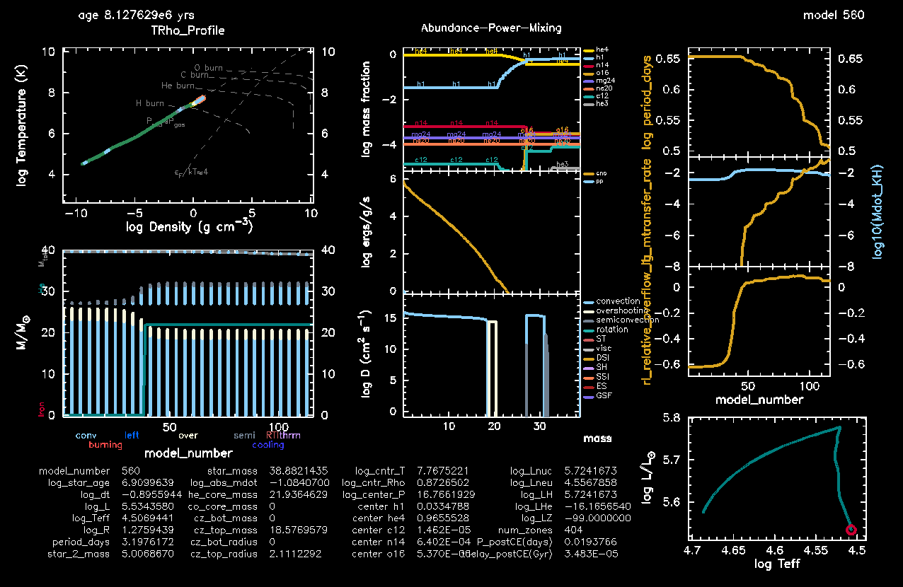
Figure 4. Common envelope evolution at its onset for a star + BH binary (click to zoom in!).
- Make sure that the Kelvin-Helmholtz rate
log10(Mdot_KH)is appearing in the plot oflg_mtransfer_rate. You can see that the threshold stays around , which gets easily surpassed by our mass transfer episode after a few models. - Make sure also the new Text Summary information on
and
from the bonus tasks are appearing:
tdelay_postCE(Gyr)andP_postCE(days). If you don’t see them, you must have missed something, but no worries. It was a long implementation! You can try to fix it, or just go to the “Discuss the run” section and simply look at Figure 4 (click to zoom in!) to answer to the conceptual questions.
Discuss the run: runaway mass transfer!
Here are some discussion points; you will only need to look at Figure 4 (click to zoom in!). Try to think about it and answer together with your table.
- How is the mass transfer rate evolving, and how can you see that you are at CE onset?
Solution
The mass transfer rate is on a steep journey of ever-growing disaster 😨 You can see it from the
lg_mtransfer_rateplot, where also we have highlighted thelog10(Mdot_KH)to show an indication of the timescale over which the star as whole fwould be able to relax thermally.You can also see it from the
rl_relative_overflowplot, in which you see a plateaux at a value above 1 (i.e. the radius of the star keeps being bigger than its Roche Lobe).
Assume now that, after CE, your system survives as a binary, and the envelope of the stripped star is fully lifted out of the system. Further, the star will quickly evolve into a BH with mass equal to its own Helium core mass. According to the energy formalism that we used to compute the post-CE properties,
Does this star + BH system produce a gravitational wave source?
Solution
Indeed, since thetdelay_postCEamounts to only 30 000 years. This will merge fast 😵💫Is the post-CE orbital period tighter in this case, with respect to the case of stable mass transfer?
Solution
Definitely tighter. In here we have something like ! As compared to the stable mass transfer cases, we have 2 order of magnitudes difference.Does this post-CE orbit make sense, i.e. could our two BHs actually fit in it?
Solution
Yes! A binary composed of black holes with masses and can physically exist with an orbital period of days. Using Kepler’s third law,
This means the two black holes orbit at a separation comparable to the radius of the Sun 🌞 For comparison, the Schwarzschild radii (a sort of indication of the BHs’ size, ) are much smaller:
- km for the BH
- km for the BH
Is the final mass ratio of your BH + BH binary different with respect to the stable mass transfer case?
Solution
The answer is yes again: the mass ratio in this case would be , much more extreme than in the stable mass transfer case.
Conclusions
Congratulations for making it till here! 🥳🥳 In this last lab we have completed our overview of binary evolution from Zero Age Main Sequence stars to binary black holes. We have learned three possible ways to form gravitational wave sources from the star + BH configuration: Case A stable mass transfer, Case B stable mass transfer, and common envelope evolution, and all three possibilites have been shown to contribute to the observed sample of gravitational waves detected by LIGO, Virgo and KAGRA interferometers1.
Important
Whether or not the relationship between star + BH remains stable determines different properties in the BH + BH resulting binary, and singling out the fingerprint of the different channels is still a hot topic: this is how the gravitational wave sources that we see today can teach us something about the (love and hate!) history of their parent stellar progenitors ♥️
References
The LIGO Scientific Collaboration, the Virgo Collaboration, the KAGRA Collaboration, et al. (2025a), GWTC-4.0: Updating the Gravitational-Wave Transient Catalog with Observations from the First Part of the Fourth LIGO-Virgo-KAGRA Observing Run ↩︎ ↩︎
Peters (1964), Gravitational Radiation and the Motion of Two Point Masses ↩︎
Lu et al. (2022), Stable mass transfer via L2 outflows in massive binaries ↩︎ ↩︎
Marchant et al. (2021), The role of mass transfer and common envelope evolution in the formation of merging binary black holes ↩︎ ↩︎
Ivanova et al. (2013), Common envelope evolution: where we stand and how we can move forward ↩︎