Lab 1: Finding the Beat
Timing: approximately 50 minutes
Learning Goals
- Install GYRE
- Set up MESA to use GYRE
- Calculate period spacing using MESA and GYRE
Scientific Background
Stars can oscillate in many different ways, much like a musical instrument. These oscillations carry information about the star’s internal structure and can therefore be used to probe regions that cannot be observed directly. Slides for all lectures can be found here: Tuesday Lecture slides
And additional slides for lab 1 can be found here: Lab 1 Background slides
Today, we focus on gravity modes (g-modes). These are oscillations for which buoyancy acts as the restoring force. G-modes propagate in stably stratified (radiative) regions of a star and are particularly sensitive to conditions near the stellar core.
Period Spacings
Each oscillation mode, with period , is characterized by a radial order , a spherical degree , and an azimuthal order . In the asymptotic limit (higher orders, where ), theory predicts that the periods should be approximately equally spaced:
In this lab, we will compute g-modes with GYRE and examine how the period spacing varies with radial order. In lab2 and lab3, you will see how chemical gradients and convective boundary mixing affect the period spacing, respectively.
Building GYRE
Your star’s personal sound system
MESA is distributed with two standalone codes for stellar oscillations:
The two codes perform broadly similar calculations, with the main tradeoff being performance versus ease of use. In this tutorial, we will focus on GYRE, which is much easier to get started with.
Getting started: download GYRE
When you downloaded MESA, the GYRE source code is included in the $MESA_DIR∕gyre directory. The official GYRE documentation is comprehensive and well maintained, and we encourage you to refer to it whenever you want more details on a particular option or output quantity. Just make sure you are viewing the documentation corresponding to the version of GYRE you are using.
Which version do you have?
For MESA version r26.4.1, the shipped GYRE version is 8.1.
You can check the version number that you have by:
ls $MESA_DIR/gyre/*.tar.gzYou will see something like
path_to_mesa/gyre/gyre-8.1.tar.gz
, where 8.1 tells you the version number.
On the website, you can change the version by clicking the small box on the right bottom corner.
Tip
We will use the version of GYRE shipped with MESA for this tutorial. However, you may wish to explore the latest release (v9.0) later, which will produce the same results but much faster. See the release notes here.
Optionally, if you would like to use the latest version of GYRE instead, download the source archive from the official website, place it wherever you like, and extract it with:
tar xf gyre-9.0.tar.gzBonding session: set environment variables
Secondly, we will set the environment variable $GYRE_DIR to the path to source directory of gyre.
export GYRE_DIR=path/to/gyreTip
If you are using the GYRE shipped with MESA, the path should be:
export GYRE_DIR=$MESA_DIR/gyre/gyreRemember that this is best placed inside your shell’s RC file in your home directory (usually .bashrc or equivalent), similarly to when you first installed MESA. Don’t forget to source this file to apply the changes to your terminal window!
Now we cook: compile
Now, we can follow the GYRE installation guide from this point. Go ahead and compile:
make -j -C $GYRE_DIR installNote
You may see linker warnings about duplicate libraries or rpath entries. These are harmless and can be safely ignored. If you encounter an error, ask a TA or developer for help.
The moment of truth: test the installation
Once compilation is complete, you should run the test suite to verify that the installation succeeded:
make -C $GYRE_DIR testImportant
If you see multiple lines indicating “…succeeded”, then everything is working correctly and you can proceed to the next step. The full test suite may take a long time, so you may let it run in the background and feel free to stop it at any time with Ctrl+C. However, it is recommended to let it finish at least once to ensure all tests pass successfully before real applications.
Running GYRE on MESA output
We will now connect GYRE to a real stellar structure model produced by MESA and compute oscillation modes.
Loaded it up: get the MESA model
In this tutorial, we will focus on the usage of GYRE, so we have prepared a simple 5 stellar model to get you started. You will learn about the setup in MESA in the next tutorial.
📋 Task: get the working directory
Download the working directory here, unzip it, and move into the folder.
💡 Hint: Unzip the file and change into the directory
unzip day2_lab1.zip
cd day2_lab1
If you are on Linux, you can use the tree . command to inspect your directory structure. Note that this command is not available by default on macOS.
You should see something like this in the folder:
.
├── 5M_at_ZAMS.mod
├── LOGS_zams
│   ├── history.data
│   ├── profile1.data
│   ├── profile1.data.FGONG
│   └── profiles.index
├── README.rst
├── clean
├── history_columns.list
├── inlist
├── inlist_pgstar
├── inlist_zams
├── make
│   └── makefile
├── mk
├── photos
│   └── x197
├── re
├── rn
└── src
    ├── run.f90
    └── run_star_extras.f90

5 directories, 18 files
Know your GYRgons: GYRE namelist
Create a file called gyre.in in your favorite text editor, and paste the following lines into this file.
&constants
/

&grid
/

&model
/

&mode
/

&num
/

&osc
/

&rot
/

&scan
/

&ad_output
/

&nad_output
/
Important
You need to add an empty line at the end of the file; otherwise GYRE will complain that the input file does not contain exactly one &nad_output namelist.
Does the structure look familiar to you?
The namelist is separated into different groups, a full explanation of the different groups and their members can be found in the documentation. In the following, we will only cover the most essential sections needed to get started.
Tip
Some namelist groups can be left empty, in which case GYRE will use the default parameter values. While this is convenient, be careful in real applications: default settings may not always match your intended configuration and can lead to unexpected results!
Grid Parameters (&grid)
This group controls the spatial resolution of the grid used by GYRE to compute oscillation modes. The grid resolution determines the spacing between adjacent points in the stellar model.
A finer grid generally improves:
- the number of modes that GYRE can successfully detect,
- and the accuracy of the computed eigenmodes.
However, increasing the number of grid points also increases the computational time.
To accurately resolve oscillation modes, the grid spacing should be smaller than the scale of the smallest significant variation in the eigenfunctions. The grid can be refined using weighting parameters such as w_osc, w_exp and w_ctr. These parameters are set to zero by default, in which case the spatial grid from the stellar model is used directly for the oscillation calculation. For our models, this default configuration is sufficient. However, higher values may be required for more realistic stellar applications.
Further details on how these parameters affect the grid can be found in the GYRE documentation here, if you need more specific control later on.
Model parameters (&model)
Here we tell GYRE what stellar model to use for computing oscillation frequencies.
📋 Task: tell GYRE the type of model to use and lead the path
Here’s the model section of the inlist with a few things missing. Use the documentation on the Model Namelist Group to determine the correct values for <MODEL_TYPE> and <PARAM>.
&model
    model_type = <MODEL_TYPE>
    <PARAM> = './LOGS_zams/profile1.data.FGONG'
    file_format = 'FGONG'
/
ℹ️ Solution
model_type tells GYRE what kind of stellar model is being used. Here, 'EVOL' indicates that we are using an evolutionary model (from MESA in our case). file pinpoints the location of the model file.
&model
    model_type = 'EVOL'
    file = './LOGS_zams/profile1.data.FGONG'
    file_format = 'FGONG'
/
file_format specifies the format of the input file. For us, it is ‘FGONG’. MESA supports various other input formats; see the full list in the table supported format.
Mode parameters (&mode)
This namelist group defines which oscillation modes you want to GYRE to search for. You can specify the angular degree ( ) and the azimuthal order ( ).
Tip
For each type of mode we will need one extra &mode namelist group.
📋 Task: Complete the Mode Namelist Group
We want the oscillation modes with
and
, and limit the radial order between -50 and -1. Search in the documentation the relevant parameters and complete the &mode namelist group.
ℹ️ Solution
&mode
    l = 1
    m = 0
    n_pg_min = -50
    n_pg_max = -1
/
Why are the radial orders negative?!!
n_pg < 0), with higher-order g modes corresponding to more negative values of n_pg. Pressure (p) modes have positive radial orders (n_pg > 0). The negative sign does not indicate a negative number of nodes; it is only used to distinguish g modes from p modes.Numerical parameters (&num)
This is where the controls for numerical aspects of calculations are set. For our simple calculation, the default settings are sufficient.
&num
    diff_scheme = 'COLLOC_GL2'
/
For most applications, you will not need to modify these settings. However, for high-precision calculations, you may wish to use higher-order differential schemes. The available diff_scheme options are listed here.
Oscillation parameters (&osc)
In this namelist group, we can configure the treatment of the stellar oscillation equations. This includes options such as the boundary conditions and the scaling factors of different physical terms in the equations.
GYRE provides many options for controlling the underlying physics of the oscillation calculations. A full list of available parameters and their default values can be found in the GYRE oscillation group documentation here.
To keep things simple, we will use the default outer boundary condition, which assumes that the density vanishes at the stellar surface:
&osc
    outer_bound = 'VACUUM'
/
Frequency Scan Parameters (&scan)
This section defines the frequency grid used by GYRE to search for oscillation modes.
Unlike the spatial grid, which discretizes the oscillation equations inside the star, the frequency grid determines the range and resolution over which GYRE searches for eigenfrequencies.
The choice of grid_type depends on the type of modes being studied:
- For p-modes, which are approximately equally spaced in frequency in the asymptotic limit, a linear frequency grid is usually preferred, i.e.,
grid_type = 'LINEAR'; - For g-modes, which are approximately equally spaced in period, an inverse-frequency grid is more appropriate, therefore,
grid_type = 'INVERSE'.
To reliably detect all modes, the scan grid spacing should generally be smaller than the separation between adjacent eigenfrequencies across the full scan range. If the grid is too coarse, some modes may be missed; if it is too fine, the runtime increases significantly. There is no universal choice for the scan parameters, and they often need to be adjusted depending on the type of modes and frequency range of interest.
📋 Task: Configure the frequency scan
Complete the &scan namelist group in gyre.in to:
- use the appropriate grid type for g-modes,
- scan frequencies between 0.1 and 10 cycles per day,
- use 500 frequency points,
- and express frequencies in cycles per day.
Search the documentation for the relevant parameter names and fill in the values.
ℹ️ Solution
&scan
    grid_type = 'INVERSE'   ! Scan grid uniform in inverse frequency
    freq_min = 0.2          ! Minimum frequency to scan from
    freq_max = 10           ! Maximum frequency to scan to
    n_freq = 500            ! Number of frequency points in scan
    freq_units = 'CYC_PER_DAY'
/
Tip
A good rule of thumb is that n_freq should be around 5 times larger than the number of modes expected to be found. Here the frequency range is provided, but in real applications this may require some experimentation.
Output parameters (&ad_output)
Finally, we need to tell GYRE what information it should save from the oscillation calculations.
GYRE provides two main types of output files:
- summary files, which contain global properties of all computed modes
- detail files, which store the eigenfunctions and structural information for individual modes.
For now, we will focus only on the summary output. Here you can include all quantities that describe the mode with a single value e.g.
,
,
, frequency, inertia, and more. A full list of available output quantities can be found in the summary files documentation. The name of the file is given by the summary_file and the quantities it should include are given with summary_item_list.
📋 Task: Settings for output files
For our purpose, we need the mode properties
,
, the radial order, and the frequency. Search in the documentation to identify the corresponding variable names, then fill the missing fields below. Also set freq_units to the proper one to remain consistent with our frequency scan.
Complete the following section in your gyre.in file (inside the &ad_output namelist). Adjust the location of your output file as you see fit.
&ad_output
    summary_file = 'summary_zams.h5'
    summary_item_list = ''
    summary_file_format = 'HDF'
    freq_units = ''
/
ℹ️ Solution
&ad_output
    summary_file = 'summary_zams.h5'
    summary_item_list = 'l,n_pg,m,freq'
    summary_file_format = 'HDF'
    freq_units = 'CYC_PER_DAY'
/
Tip
The output settings are placed inside the &ad_output namelist group, indicating that we are performing an adiabatic oscillation calculation. If we want to instead calculate it non-adiabatically we would need to put it in &nad_output instead.
Putting it all together
One last check
Before we proceed to run GYRE, you might check that you have everything in place.
The final look of our gyre.in
&constants
/

&model
    model_type = 'EVOL'
    file = './LOGS_zams/profile1.data.FGONG'
    file_format = 'FGONG'
/

&mode
    l = 1
    m = 0
    n_pg_min = -50
    n_pg_max = -1
/

&osc
    outer_bound = 'VACUUM'
/

&scan
    grid_type = 'INVERSE'
    freq_min = 0.2
    freq_max = 10
    n_freq = 500
    freq_units = 'CYC_PER_DAY'
/

&rot
/

&grid
/

&num
    diff_scheme = 'COLLOC_GL2'
/

&ad_output
    summary_file = 'summary_zams.h5'
    summary_item_list = 'l,n_pg,m,freq'
    summary_file_format = 'HDF'
    freq_units = 'CYC_PER_DAY'
/

&nad_output
/
GYRE it up
Now you are all set! Go ahead and run GYRE:
$GYRE_DIR/bin/gyre gyre.inTip
If you run GYRE frequently, you can create an alias by adding the following line in your bash.rc (or equivalent) so that you can simply run gyre gyre.in and save some typing.
alias gyre="$GYRE_DIR/bin/gyre"What do you see on screen?
If everything goes as planned, you would see that information on loading the stellar model, building the spatial and frequency grids, and then searching for oscillation modes for = 1, = 0.
Each line in the table corresponds to one detected mode and lists:
n_pg: radial order (negative here → g-modes)n_p,n_g: p- and g-mode node countsRe(omega): oscillation frequency of the modeIm(omega): growth/damping rate (zero here → stable, adiabatic modes)chi+n_iter: convergence diagnostics for the root solver
A simple sanity check when running GYRE is that n_pg increases strictly by 1. If this is not the case, it usually signals an issue. The troubleshooting section is a good place to look for possible causes.
See the beat
We have prepared a Google Colab for you to visualize your model. Before editing the notebook, save a copy to your own Google Drive (File → Save a copy in Drive), otherwise your changes may not persist.
Prefer to work locally?
The easiest way to visualize GYRE output is with the Python package pygyre, available on the Python Package Index (PyPI).
Important
It is preferable to create a separate Python environment so that dependencies do not conflict with other projects.
If you have the Python package manager pip, you can install it with:
pip install pygyreOnce pygyre is installed, you can download the notebook and work locally. Remember to skip the first cell (!pip install ...) in this case.
📋 Task: plot the period spacing
Upload your summary file to the Google Colab, and plot the period spacing. What do you expect to see?
If you encountered issues producing the summary file, you can download it here.
📈 period spacing
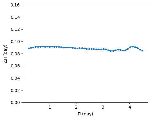
The period spacings are almost constant!
In the asymptotic limit (high radial order), g-modes period spacings are nearly constant. Deviations from a constant period spacing provide valuable information about the stellar interior, such as chemical gradients, convective boundaries, or rotation.
Bonus: more diagnostic from the detail files
As mentioned before, in addition to the summary files, GYRE can have another type of output files called detail files. The detail files provide additional information about individual modes, such as eigenfunctions and propagation properties.
To tell GYRE to output the detail files, add the following lines in the &ad_output section:
&ad_output
    ....

    detail_template = 'detail_zams/detail.l%l.n%n.h5'
    detail_item_list = 'l,n_pg,omega,freq,x,xi_r,xi_h,c_1,As,V_2,Delta_g,Gamma_1,rho'
/
Important
GYRE creates one detail file per mode, so the number of output files can grow quickly. To keep things organized, it is convenient to store them in a separate folder.
However, GYRE does not create directories automatically, so you must create the folder yourself before running GYRE. Name it, for example, detail_zams:create a subfolder
mkdir detail_zams
The %l and %n will be replaced by the harmonic degree
and the radial order
, respectively. For more options, check out the doc. The detail_item_list specifies the quantities we are interested in.
Again,
$GYRE_DIR/bin/gyre gyre.inNow if you do:
ls -l detail_zams/* | wc -lYou will see the number of the modes found by GYRE.
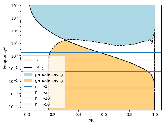
📋 Bonus task: inspect the propagation diagram
The propagation diagram is basically a “map” showing where different types of waves can and cannot travel inside a star. The Brunt–Väisälä frequency ( ) and the Lamb frequency ( ) set the boundaries of the propagation regions: gravity waves propagate where (g mode cavity), while pressure waves propagate where (p mode cavity).
Go to the Google Colab, upload one of your detail files there, and use the provided plotting function plot_propagation_diagram to plot the propagation diagram.
If you encounter issues producing the detail files, we have prepared the ones for n_pg=-1, n_pg=-25, and n_pg=-45, also discuss with others to see what they get.
📈 propagation diagram
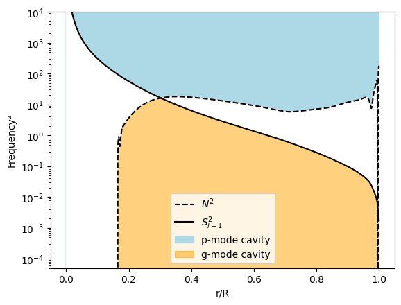
Here, one sees the p-mode and g-mode cavities separated by the Lamb (solid) and Brunt–Väisälä (dashed) frequency profiles.
By looking at the position of modes on the propagation diagram, one can determine whether a mode can propagate or is evanescent in different regions. In this case, all the modes lie in regions where propagation is allowed.📈 how modes are placed on the propagation diagram
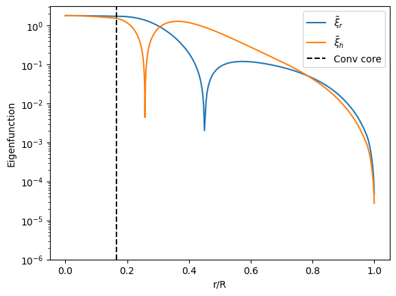
📋 Bonus task: inspect the displacement eigenfunctions
One can inspect the eigenfunctions of each mode through the detail files. Upload a few detail files to the Google Colab notebook and use the provided plotting functions to inspect the radial (xi_r) and horizontal (xi_h) displacement eigenfunctions of different modes.
Compare how the eigenfunctions change with radial order.
📈 eigenfunctions
For n_pg = -1:
For n_pg = -50:
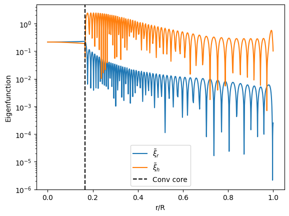
and are the radial and horizontal displacement perturbations, respectively.
Inside the convective core, the radial and horizontal displacement amplitudes are of the same order because convection produces nearly isotropic, turbulent motions with no strong restoring buoyancy stratification. As a result, oscillatory motions are not strongly constrained into a preferred direction. Outside the convective core, in the stably stratified radiative region, radial motions are strongly restored by buoyancy, so horizontal motions dominate. This is characteristic of g mode propagation.
Bonus: A short introduction to how GYRE finds oscillation modes
GYRE solves the stellar oscillation equations, a set of differential equations and boundary conditions that describe small, periodic perturbations about a star’s equilibrium state. Consistent solutions to these equations (known as “modes”) can be found only for certain specific choices of the perturbation frequency, and so the frequency takes on the mathematical role of an eigenvalue.
To calculate the frequency eigenvalues (or “eigenfrequencies”) of a stellar model (obtained, for instance, from MESA), GYRE sets up a large system of algebraic equations. These equations are derived from finite-difference approximations to the oscillation differential equations, taken between pairs of adjacent spatial grid points. In symbolic form, the algebraic equations can be written as
where is a matrix of coefficients and is a vector of unknowns representing the perturbations at each grid point. Solutions to this equation only exist when
and so GYRE’s task is to search for the frequencies at which the determinant of vanishes. Once these eigenfrequencies are found, GYRE reconstructs the associated eigenfunctions (describing the spatial dependence of perturbations) from the vector .
The eigenfrequencies of a star depend on the detailed internal structure of the star. Therefore, by comparing a set of eigenfrequencies for a given stellar model against those observed in a real star, we can test how well the model represents the real star — a technique known as asteroseismology.
Reference
Solution
The complete solution is available here.
Acknowledgement:
- This tutorial is largely inspired by similar labs for the 2025 MESA Summer School and the GYRE documentation.
- The short introduction to how GYRE finds oscillation modes is written by Meng Sun and proofread by Rich Townsend.