Minilab 2: Getting in Debt
Introduction
In Lab 1 you built a minimal nuclear network for an accreting ONe white dwarf and watched the core march toward oxygen ignition. But there is important physics we left out: the Urca process.
In sufficiently degenerate matter, certain nuclei can undergo cyclic electron captures and beta decays at a specific threshold density — a so-called Urca shell. The name comes from the Urca Casino in Rio de Janeiro: neutrinos carry energy out of the star as quickly as money vanishes at the tables. Each cycle emits two neutrinos, providing a potentially significant cooling mechanism that is sensitive to the accretion rate.
In this lab you will:
- Add the A=23 Urca pair ( ↔ ) to your nuclear network and observe the Urca shell in real time with pgstar.
- Add the A=25 Urca pair ( ↔ ↔ ) and compare its effect against the A=23 run using pgstar plots and terminal history output.
- Estimate the compressional heating and Urca cooling timescales of the white dwarf.
The files for this lab can be found in the Lab 2 Google Drive folder (starting point, partial solutions, and full solution).
Consult the MESA documentation throughout this lab.
Part 1: Adding the A=23 Urca Pair (²³Na/²³Ne)
Step 0: Start Up
| 📋 TASK 1 |
|---|
| Download the Lab 2 starting point from the Google Drive and unzip it to a local working directory. |
The starting point is similar to your completed Lab 1 setup, but now configured to load a 1.1 M☉ O-Ne-Na white dwarf model.
After downloading, your working directory should look like:
- clean
- mk
- re
- rn
- history_columns.list
- profile_columns.list
- inlist
- inlist_common
- inlist_accrete
- inlist_pgstar
- ONe.net
- 1.1Msun_ONeNa.mod
- 1.1Msun_ONeMg2Na.mod
- run.f90
- run_star_extras.f90
Note
run_star_extras.f90 has been updated from Lab 1. It now computes the A=23 electron capture and beta decay rates (
and
) as extra profile columns used by pgstar to show the Urca shell.
Tip
After unzipping, verify your directory matches the listing above by running ls (Linux/Mac) or dir (Windows) in the working directory.
Step 1: Build the ONeNa Network
A nuclear network defines which isotopes and reactions MESA tracks during a simulation. By default, reactions not in the network are ignored even if they could occur at the conditions being modelled. To study the A=23 Urca shell we need the network to know about and and the weak reactions connecting them.
The starting network (ONe.net) contains the ²⁰Ne→²⁰F→²⁰O electron capture chain and ¹⁶O burning, but no ²³Na or ²³Ne.
To model the A=23 Urca pair we need to add both isotopes and their connecting weak reactions.
| 📋 TASK 2 |
|---|
Create a new file ONeNa.net in your working directory. Starting from ONe.net, add
,
and the two Urca reactions that connect them. |
Note
MESA reaction names follow the pattern r_<lhs>_wk_<rhs> (electron capture) and r_<lhs>_wk-minus_<rhs> (beta decay). A full list of available weak reactions can be found under $MESA_DIR/data/rates_data/weakreactions.tables.
Note
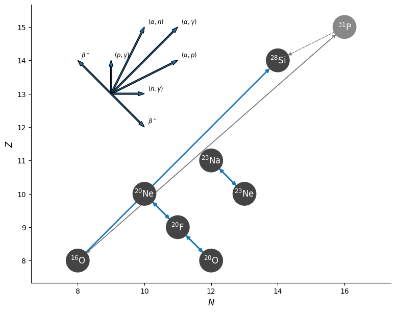
The A=23 Urca pair consists of:
- Electron capture:
- Beta decay:
Visually this network look like:
Hint: What isotopes and reactions to add?
Add to add_isos(...):
na23ne23
Add to add_reactions(...):
r_na23_wk_ne23— electron capture Na23 + e⁻ → Ne23r_ne23_wk-minus_na23— beta decay Ne23 → Na23 + e⁻
Partial Solution
add_isos(
    h1
    he4
    o16
    ! for Ne20 - F20 - O20 electron capture chain
    ne20
    f20
    o20
    ! for A=23 Urca pair
    na23
    ne23
    ! for O ignition
    si28
    )

add_reactions(
    ! for oxygen ignition
    r1616
    ! for Ne20 - F20 - O20
    r_ne20_wk_f20
    r_f20_wk-minus_ne20
    r_f20_wk_o20
    r_o20_wk-minus_f20
    ! A=23 Urca pair: Na23 + e- <-> Ne23
    r_na23_wk_ne23
    r_ne23_wk-minus_na23
    )
Step 2: Update the Inlists
With the network in hand, update the inlists to use it and include in the accreted material.
| 📋 TASK 3 |
|---|
In inlist_accrete, change the network to ONeNa.net and add Na²³ to the accreted composition. Use a mass fraction of 5%
(reducing
from 50% to 45%). |
Hint: What variables need to be changed?
In &star_job:
new_net_name = 'ONeNa.net'
In &controls, update the accretion block:
num_accretion_species = 3- Add
accretion_species_id(3) = 'na23'andaccretion_species_xa(3) = 0.05d0 - Adjust fraction so that all fractions sum to 1.
Partial Solution
! in &star_job
    new_net_name = 'ONeNa.net'   !!!!!

! in &controls
    num_accretion_species = 3           !!!!!
    accretion_species_id(1) = 'o16'
    accretion_species_xa(1) = 0.50d0
    accretion_species_id(2) = 'ne20'
    accretion_species_xa(2) = 0.45d0   !!!!!
    accretion_species_id(3) = 'na23'   !!!!!
    accretion_species_xa(3) = 0.05d0   !!!!!
Step 3: Run and Observe the A=23 Urca Shell
| 📋 TASK 4 |
|---|
Compile and run with ./clean, ./mk then ./rn. In the pgstar window labelled “A=23 Urca Shell”, observe the composition profile and the neutrino emissivity as the core density increases. |
You should see two windows open: the main grid overview (Grid2) and the Urca shell profile plot (Profile_Panels1).
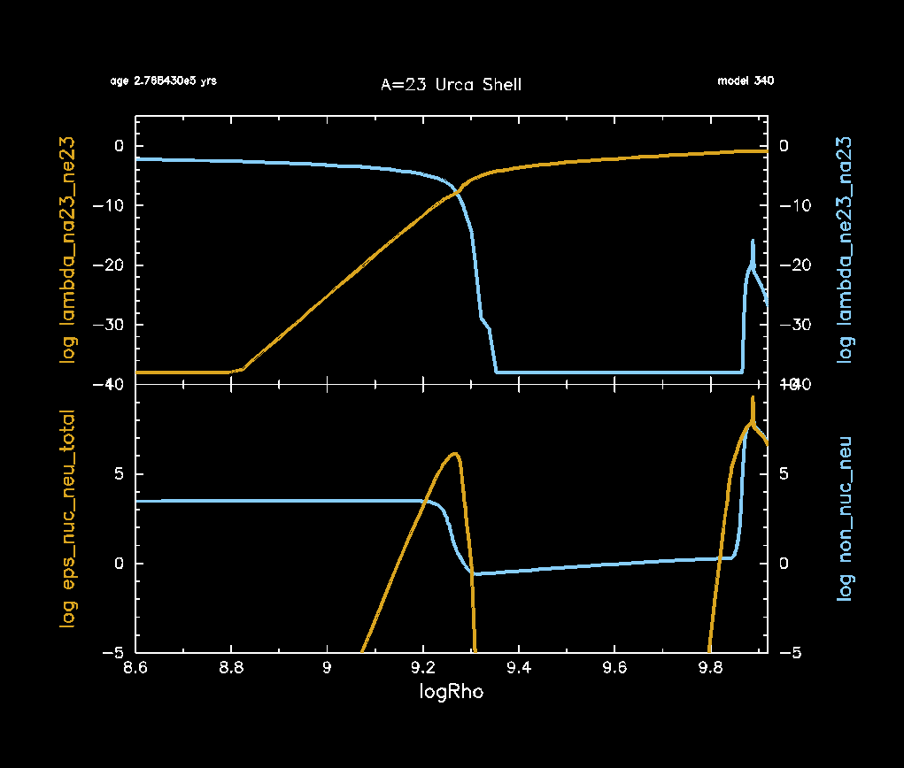
In Profile_Panels1, look for:
- Top panel — the electron capture rate ( ) and beta decay rate ( ) as functions of . The Urca shell is located where these two rates are equal ( ), corresponding to the threshold density.
- Bottom panel — the neutrino emissivity (
eps_nuc_neu_total, solid) and thermal neutrino emission (non_nuc_neu, dashed). A localised peak in the nuclear neutrino emissivity marks the active Urca shell.
Tip
PNG snapshots of each pgstar frame are saved to png/ inside your LOGS directory. If you miss a frame or want to compare later, check there.
Note
At what log density does the A=23 Urca shell sit? You can compare this to the theoretical threshold:
What if pgstar shows nothing in the Profile_Panels1 window?
log_cntr_Rho in the text summary to track progress.Note
If you want to see the final pgstar frame before MESA closes, you can add pause_before_terminate = .true. to the &star_job section of inlist_common.
Part 2: Adding the A=25 Urca Pair (²⁵Mg/²⁵Na/²⁵Ne)
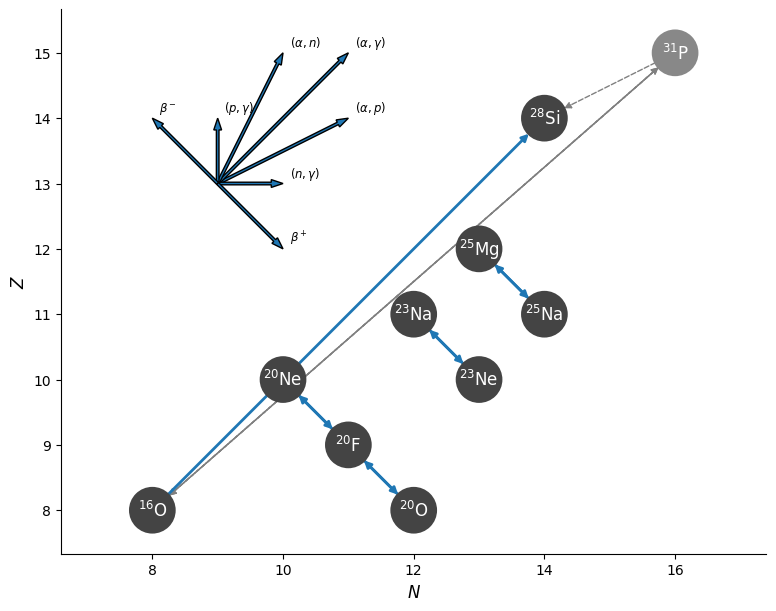
The A=25 Urca pairs operate at different threshold densities than A=23. It consists of a two-step electron capture chain:
and the reverse beta decays.
Visually, this network appears as:
Step 4: Build the ONeNaMg25 Network
ONeMg white dwarfs accrete material that includes and from their envelopes. undergoes a two-step electron capture chain at densities slightly above the A=23 Urca shell, making it the next natural Urca pair to add. does not have an Urca pair in this density range but is still accreted and should be tracked.
| 📋 TASK 5 |
|---|
Create a new file ONeNaMg25.net by extending ONeNa.net to include the A=25 species and reactions. Also add
as a tracked species (it is accreted). |
Hint: What isotopes and reactions to add?
Additional isotopes:
mg25,na25,ne25mg24(tracked; no new Urca reactions needed for A=24 at this stage)
Additional reactions:
r_mg25_wk_na25— EC: Mg25 + e⁻ → Na25r_na25_wk-minus_mg25— BD: Na25 → Mg25 + e⁻r_na25_wk_ne25— EC: Na25 + e⁻ → Ne25r_ne25_wk-minus_na25— BD: Ne25 → Na25 + e⁻
Partial Solution
add_isos(
    h1
    he4
    o16
    ne20
    f20
    o20
    ! A=23 Urca pair
    na23
    ne23
    ! A=25 Urca pair
    mg25
    na25
    ne25
    ! other accreted species
    mg24
    ! for O ignition
    si28
    )

add_reactions(
    r1616
    ! Ne20 - F20 - O20
    r_ne20_wk_f20
    r_f20_wk-minus_ne20
    r_f20_wk_o20
    r_o20_wk-minus_f20
    ! A=23 Urca pair
    r_na23_wk_ne23
    r_ne23_wk-minus_na23
    ! A=25 Urca pair
    r_mg25_wk_na25
    r_na25_wk-minus_mg25
    r_na25_wk_ne25
    r_ne25_wk-minus_na25
    )
Step 5: Update the Inlists for the A=25 Run
Note
The 1.1Msun_ONeMg2Na.mod starting model is already included in your working directory.
| 📋 TASK 6 |
|---|
Update inlist_accrete to use ONeNaMg25.net, load the 1.1Msun_ONeMg2Na.mod starting model, set the LOGS directory to LOGS_ONeNaMg25_1d-6, and update the accretion composition to include ²⁴Mg (5%) and ²⁵Mg (1%). |
Note
We want all accreted mass fractions to sum to 1. Adding Mg24 (5%) and Mg25 (1%) means reducing something else by 6%. We reduce Ne: it is the most abundant species in the mix, and because Ne ignites (via electron capture) at a higher density than O, its exact initial abundance matters less for the dynamics we are studying here. The true initial composition of an ONe white dwarf would need to be determined through full stellar evolution calculations.
Partial Solution
! in &star_job
    load_model_filename = '1.1Msun_ONeMg2Na.mod'                                !!!!!
    new_net_name = 'ONeNaMg25.net'                                !!!!!

! in &controls
    num_accretion_species = 5           !!!!!
    accretion_species_id(1) = 'o16'
    accretion_species_xa(1) = 0.50d0
    accretion_species_id(2) = 'ne20'
    accretion_species_xa(2) = 0.39d0   !!!!!  (reduced from 0.45 to make room for Mg24+Mg25)
    accretion_species_id(3) = 'na23'
    accretion_species_xa(3) = 0.05d0
    accretion_species_id(4) = 'mg24'   !!!!!
    accretion_species_xa(4) = 0.05d0   !!!!!
    accretion_species_id(5) = 'mg25'   !!!!!
    accretion_species_xa(5) = 0.01d0   !!!!!

log_directory = 'LOGS_ONeNaMg25_1d-6' !!!!!| 📋 TASK 7 |
|---|
In src/run_star_extras.f90, extend the rate computation to include the A=25 pair: change to 4 profile columns and add the Mg25/Na25 species pair. Recompile with ./clean && ./mk. |
Hint: run_star_extras.f90 — changes for A=25 rates
In how_many_extra_profile_columns, change 2 to 4.
In data_for_extra_profile_columns, extend nr, the column names, and the species pairs:
! Change:
how_many_extra_profile_columns = 4

! In data_for_extra_profile_columns:
names(1) = 'lambda_na23_ne23'
names(2) = 'lambda_ne23_na23'
names(3) = 'lambda_mg25_na25'    ! A=25 EC: Mg25 + e- -> Na25
names(4) = 'lambda_na25_mg25'    ! A=25 BD: Na25 -> Mg25 + e-

nr = 4     ! was 2
! allocate(...) call stays the same — nr now controls the size

weak_lhs(1) = 'na23'; weak_rhs(1) = 'ne23'
weak_lhs(2) = 'ne23'; weak_rhs(2) = 'na23'
weak_lhs(3) = 'mg25'; weak_rhs(3) = 'na25'
weak_lhs(4) = 'na25'; weak_rhs(4) = 'mg25'| 📋 TASK 8 |
|---|
In inlist_pgstar, expand Profile_Panels1 to 3 panels: A=23 rates (panel 1), A=25 rates (panel 2), and the neutrino emissivity (panel 3). No recompile needed. |
Hint: inlist_pgstar — expand to 3 panels
Change profile_panels1_num_panels = 2 to 3 and update the title.
Insert a new panel 2 block for the A=25 rates, and update the neutrino emissivity block from index (2) to (3):
profile_panels1_num_panels = 3
profile_panels1_title = 'Urca Shells'

! Panel 2: A=25 pair — Mg25 e-capture (left axis) vs Na25 beta-decay (right axis)
profile_panels1_yaxis_name(2) = 'lambda_mg25_na25'
profile_panels1_yaxis_log(2) = .true.
profile_panels1_ymin(2) = -40d0
profile_panels1_ymax(2) = 5d0
profile_panels1_other_yaxis_name(2) = 'lambda_na25_mg25'
profile_panels1_other_yaxis_log(2) = .true.
profile_panels1_other_ymin(2) = -40d0
profile_panels1_other_ymax(2) = 5d0

! Panel 3: neutrino emissivity — change all (2) indices below to (3)
profile_panels1_yaxis_name(3) = 'eps_nuc_neu_total'
profile_panels1_yaxis_log(3) = .true.
profile_panels1_ymin(3) = -5d0
profile_panels1_ymax(3) = 10d0
profile_panels1_other_yaxis_name(3) = 'non_nuc_neu'
profile_panels1_other_yaxis_log(3) = .true.
profile_panels1_other_ymin(3) = -5d0
profile_panels1_other_ymax(3) = 10d0
Step 6: Run and Compare with pgstar
| 📋 TASK 9 |
|---|
Run the A=25 case (./rn) and observe the Profile_Panels1 window — it now shows three panels: A=23 rates (panel 1), A=25 rates (panel 2), and the combined neutrino emissivity (panel 3). |
Look for:
- A second Urca shell appearing at a lower density than the A=23 shell, and a third shell appearing at a higher density than the A=23 shell.
- Any change in the neutrino emissivity profile — do the A=25 shells contribute noticeably?
Tip
If you want to compare frames from the two runs side-by-side, check the png/ subdirectory inside each LOGS directory. MESA saves a PNG of every pgstar frame there.
Note
Theoretical threshold density for the A=25 shells:
Step 7: Compare the Two Runs
| 📋 TASK 10 |
|---|
Compare your A=23-only run against the A=23+A=25 run. Open the png/ subdirectory inside each LOGS directory and compare the final pgstar frames side-by-side. Look at the central temperature and density evolution — does adding the second Urca pair produce a noticeable difference in the thermal history? |
Things to compare:
- Central temperature and density at the end of the run.
- Neutrino luminosity (
log_Lneu) from your history file. - The density at which the A=25 Urca shell becomes active compared to A=23.
Discussion: what to expect
Bonus: Compressional Heating and Urca Cooling Timescales
Note
For background on the physics in this bonus section, see Appendix A of Schwab et al. 2017.
As the white dwarf accretes mass, compressional work heats the core. The Urca shells remove this energy via neutrinos. The competition between these rates governs the thermal evolution and ultimately the ignition conditions.
Three timescales capture this competition:
| Symbol | Formula | Physical meaning |
|---|---|---|
| How long it takes to compress the core by -fold | ||
| Time for the core to sweep through the Urca shell (shell width in ) | ||
| Thermal energy content divided by neutrino loss rate |
Here
is the electron degeneracy parameter and
is the net neutrino energy loss rate per gram.
These timescales can be computed using variables stored in the star_info pointer s at each timestep.
Bonus Step 1: Add timescale history columns
MESA lets you log custom quantities by implementing two functions in run_star_extras.f90:
how_many_extra_history_columns— returns the number of extra columnsdata_for_extra_history_columns— fills in the column names and values
Open src/run_star_extras.f90. You will find both functions already stubbed out (the history counterparts of the profile lambda columns you added in Part 1). The stub looks like:
integer function how_many_extra_history_columns(id)
   ...
   how_many_extra_history_columns = 0   ! !!!!! bonus: change to 3
end function how_many_extra_history_columns

subroutine data_for_extra_history_columns(id, n, names, vals, ierr)
   integer, intent(in) :: id, n
   character (len=maxlen_history_column_name) :: names(n)
   real(dp) :: vals(n)
   ...
   ! !!!!! bonus: fill in names and values here
end subroutine data_for_extra_history_columns
The three timescales require quantities evaluated at a single zone. We use zone index s% nz, which is the innermost zone (the stellar centre). All per-zone quantities in star_info are arrays indexed by zone; using s% nz picks out the central value:
| Field | Units | Quantity |
|---|---|---|
s% dt | s | Current timestep |
s% dxh_lnd(s% nz) | — | over this step |
s% eta(s% nz) | — | Electron degeneracy parameter |
s% cv(s% nz) | erg g⁻¹ K⁻¹ | Heat capacity at constant volume |
s% T(s% nz) | K | Temperature |
s% eps_nuc_neu_total(s% nz) | erg g⁻¹ s⁻¹ | Net neutrino energy loss rate |
secyer | s yr⁻¹ | Seconds per year (from const_def, already used) |
| 📋 BONUS TASK 1 |
|---|
In run_star_extras.f90, change how_many_extra_history_columns to return 3. Then populate data_for_extra_history_columns with names and computed values for 'tau_rho', 'tau_cross', and 'tau_cool' (output in years). Recompile with ./mk. |
Hint: code for data_for_extra_history_columns
subroutine data_for_extra_history_columns(id, n, names, vals, ierr)
   ...
   real(dp) :: tau_rho, tau_cross, tau_cool

   names(1) = 'tau_rho'
   names(2) = 'tau_cross'
   names(3) = 'tau_cool'

   ! tau_rho: compressional timescale
   tau_rho = s% dt / max(abs(s% dxh_lnd(s% nz)), 1d-99)
   vals(1) = tau_rho / secyer

   ! tau_cross: time to sweep through the Urca shell
   tau_cross = 9d0 / max(s% eta(s% nz), 1d-10) * tau_rho
   vals(2) = tau_cross / secyer

   ! tau_cool: neutrino cooling timescale
   if (s% eps_nuc_neu_total(s% nz) > 0d0) then
      tau_cool = s% cv(s% nz) * s% T(s% nz) / s% eps_nuc_neu_total(s% nz)
   else
      tau_cool = 1d99
   end if
   vals(3) = min(tau_cool / secyer, 1d99)
The max(...) guards prevent division by zero during the early stages of a run.
Bonus Step 2: Display the timescales in pgstar
MESA’s History_Panels plot type can display any history column (including your new extras) against any other history column or model number.
Each panel has a left and right y-axis; set yaxis_log = .true. to display
of the value.
Add a History_Panels1 block to inlist_pgstar that shows the three timescales vs
— no recompile needed.
| 📋 BONUS TASK 2 |
|---|
Add a History_Panels1 window to inlist_pgstar with 2 panels: one comparing
and
, another comparing
and
. Use log_center_Rho as the x-axis. Run with ./rn and watch the timescales evolve. |
Hint: inlist_pgstar controls
  History_Panels1_win_flag = .true.
  History_Panels1_win_width = 10
  History_Panels1_title = 'Timescales'

  History_Panels1_xaxis_name = 'log_center_Rho'
  History_Panels1_xmin = 8.5d0
  History_Panels1_xmax = -101d0   ! -101 means auto

  History_Panels1_num_panels = 2

  ! Panel 1: compressional vs cooling
  History_Panels1_yaxis_name(1) = 'tau_rho'
  History_Panels1_yaxis_log(1) = .true.
  History_Panels1_ymin(1) = 0d0
  History_Panels1_ymax(1) = 15d0
  History_Panels1_other_yaxis_name(1) = 'tau_cool'
  History_Panels1_other_yaxis_log(1) = .true.
  History_Panels1_other_ymin(1) = 0d0
  History_Panels1_other_ymax(1) = 15d0

  ! Panel 2: crossing vs cooling
  History_Panels1_yaxis_name(2) = 'tau_cross'
  History_Panels1_yaxis_log(2) = .true.
  History_Panels1_ymin(2) = 0d0
  History_Panels1_ymax(2) = 15d0
  History_Panels1_other_yaxis_name(2) = 'tau_cool'
  History_Panels1_other_yaxis_log(2) = .true.
  History_Panels1_other_ymin(2) = 0d0
  History_Panels1_other_ymax(2) = 15d0
Bonus Step 3: Interpret the results
| 📋 BONUS TASK 3 |
|---|
Run with ./rn. At late times (
), which timescale is shortest:
,
, or
? What does the ordering imply for whether the Urca shells can efficiently regulate the core temperature? |
Discussion hint
- If : the Urca shells cool the WD faster than compression heats it — the core temperature plummets.
- If : compressional heating wins and the WD warms up.
This balance is sensitive to and the Urca pair threshold densities — exactly the crowdsourcing question you will explore in Lab 3!
Solution / End Point
The end-of-Part-2 solution for Lab 2 (which also serves as a starting point for Lab 3) can be downloaded HERE.
If you also completed the bonus section, the full bonus solution can be downloaded HERE.